Machine Learning Specialization: Arjunan K
Detailed notes of Machine Learning Specialization by Andrew Ng in collaboration between DeepLearning.AI and Stanford Online in Coursera, Made by Arjunan K.
Supervised Machine Learning: Regression and Classification - Course 1
Intro to Machine Learning
Machine Learning is the Ability of computers to learn without being explicitly programmed. There are different types of Machine Learning Algorithms.
- Supervised Learning
- Unsupervised Learning
- Recommender Systems
- Reinforcement Learning
Supervised Learning
Machines are trained using well "labelled" training data, and on basis of that data, machines predict the output. The labelled data means some input data is already tagged with the correct output. It find a mapping function to map the input variable(x) with the output variable(y). Some use cases are given below,
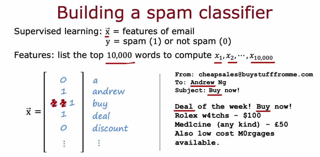
- Spam Filtering
- Speech Recognition
- Text Translation
- Online Advertising
- Self-Driving Car
- Visual Inspection (Identifying defect in products)
Types of Supervised Learning
- Regression
- Classification
Unsupervised Learning
Models are not supervised using labelled training dataset. Instead, models itself find the hidden patterns and insights from the given data. It learns from un-labelled data to predict the output.
Types of Unsupervised Learning
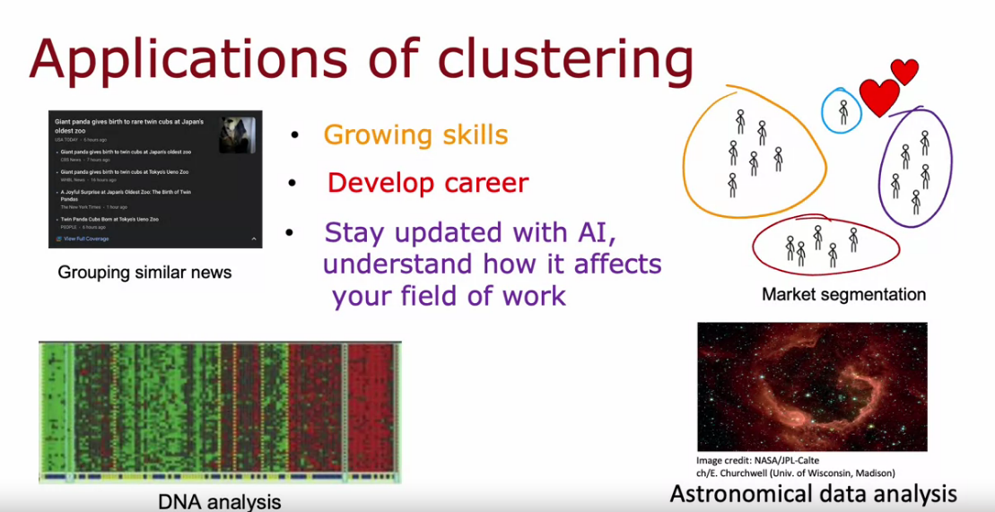
- Clustering (Group similar data like DNA, Customer, Disease Features)
- Anomaly Detection (Finds unusual data points)
- Dimensionality Reduction (Compress data to fewer numbers)
REGRESSION
It’s used as a method for predictive modelling in machine learning in which an algorithm is used to predict continuous outcomes. Commonly used regression is
Linear Regression
- Simple Linear Regression - (one dependent and one independent variable)
- Multiple linear regression - (one dependent and multiple independent variable)
CLASSIFICATION
It predicts categories, the program learns from the given dataset or observations and then classifies new observation into a number of classes or groups. Such as, Yes or No, 0 or 1, Spam or Not Spam, cat or dog etc. Classes can be called as targets/labels or categories. Commonly used classification is
Logistic Regression
In this note we will be focusing on the math behind the Linear and Logistic Regression Models.
SIMPLE LINEAR REGRESSION
- It is fitting a straight line to your data.
- Model the relation between independent (Input X) and dependent (Output Y) by fitting a linear equation to observed data.
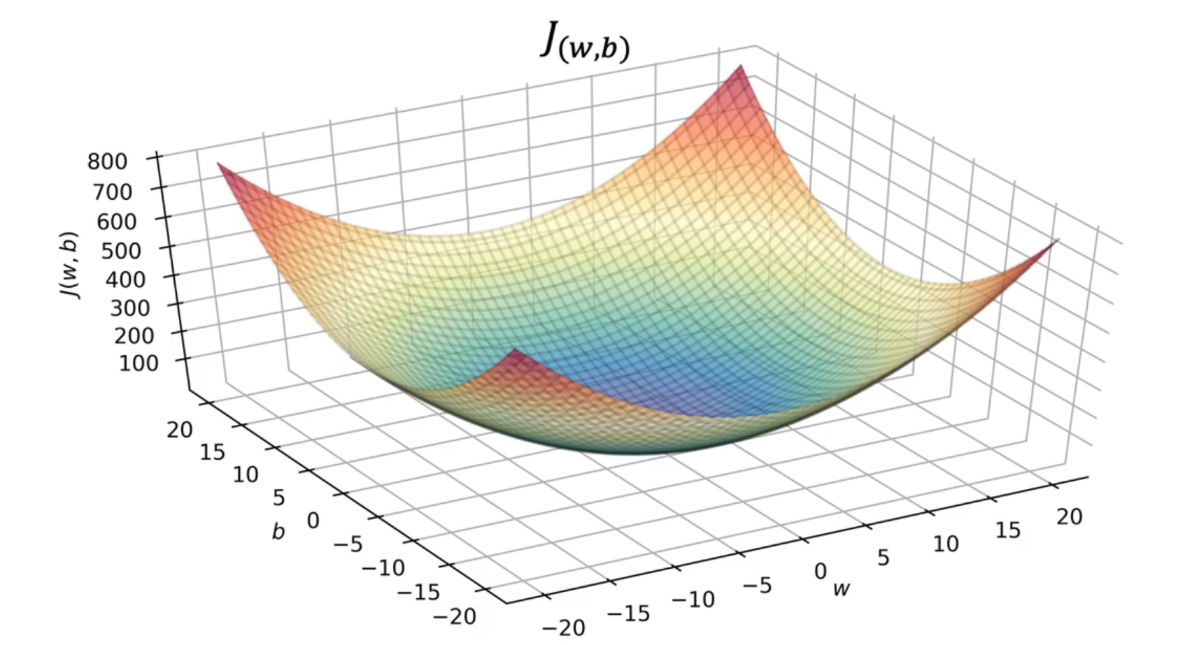
What is Cost Function?
A cost function is an important parameter that determines how well a machine learning model performs for a given dataset. It calculates the difference between the expected value and predicted value and represents it as a single real number. It is the average of loss function (Difference between predicted and actual value).
Our aim is to minimize the cost function, which is achieved using Gradient Descent.
Types of cost function.
- Mean Squared Error (MSE) for Linear Regression
- Log Loss for Logistic Regression
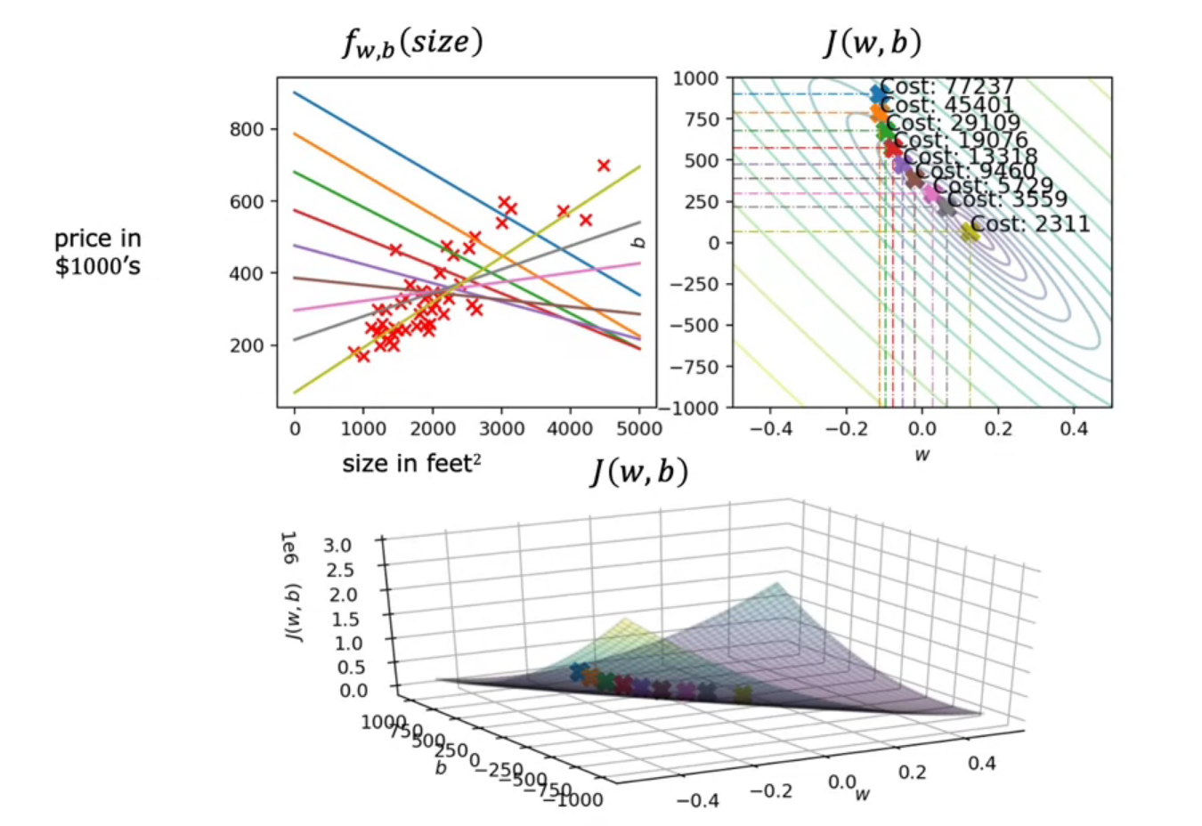
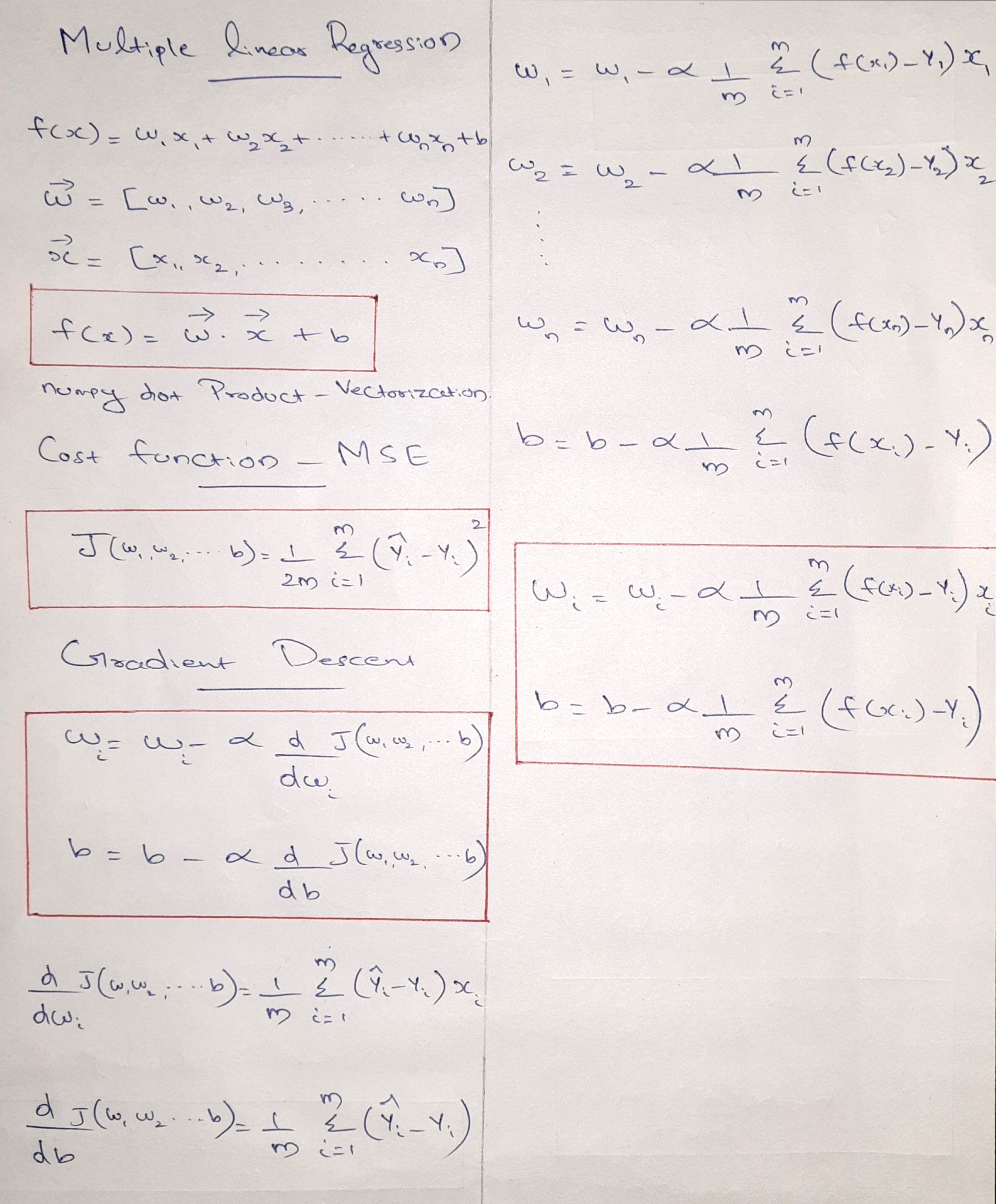
Cost Function for Linear Regression - MSE (Convex)
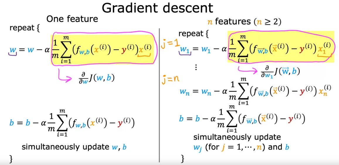
Gradient Descent
Gradient descent is an optimization algorithm which is commonly-used to train machine learning models and neural networks. Training data helps these models learn over time, and the cost function within gradient descent specifically acts as a barometer, gauging its accuracy with each iteration of parameter updates. Until the function is close to or equal to zero, the model will continue to adjust its parameters to yield the smallest possible error. We start with
Normal Equation (Alternative for Gradient Descent)
- Only for Linear Regression
- Solve w and b without iteration.
- But not a generalized one for other learning algorithm.
- when number of features is large > 1000, it is slow.
- most libraries use this under the hood.
- but gradient is better and general.
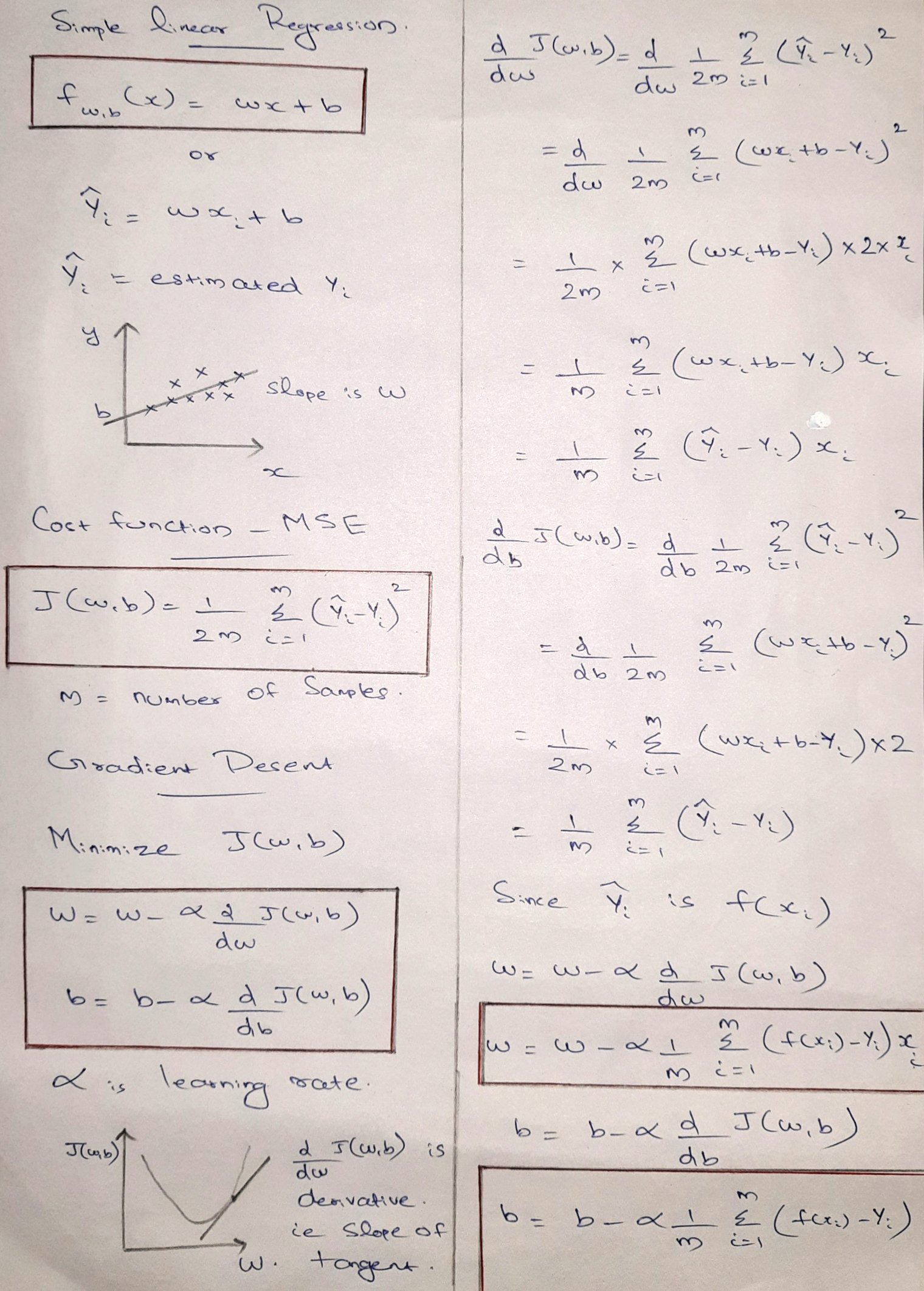
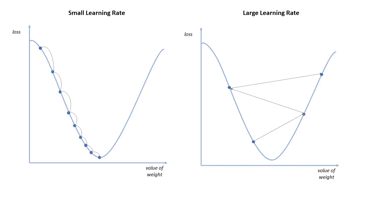
Learning Rate
The learning rate is a hyperparameter that controls how much to change the model in response to the estimated error each time the model weights are updated.
- Small learning rate may result slow gradient descent.
- Large learning rate may result in divergence of descent (Fail to converge to minimum).
- If the cost function reaches local minimum, slope become zero. So w = w, not going to descent after that.
- Fixed learning rate has no problem, since derivative part decrease as we decent.
- Alpha value can be 0.001 and increased 3X times based on requirement. If Cost function is increasing decrease Alpha and Vice Versa.
1. Batch gradient descent (Used in this course)
Each step of gradient descent uses all training data. This process referred to as a training epoch.
2. Stochastic gradient descent
Each step of gradient descent uses a subset of training data. It runs a training epoch for each example within the dataset and it updates each training example's parameters one at a time.
3. Mini-batch gradient descent
Mini-batch gradient descent combines concepts from both batch gradient descent and stochastic gradient descent. It splits the training dataset into small batch sizes and performs updates on each of those batches. This approach strikes a balance between the computational efficiency of batch gradient descent and the speed of stochastic gradient descent.
Multiple Linear Regression
- Here we predict one dependent variable from multiple independent variable.
SIMPLE v/s MULTIPLE
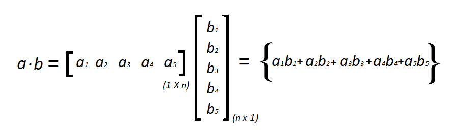
WHAT IS VECTORIZATION?
Vectorization is used to speed up the code without using loop. Using such a function can help in minimizing the running time of code efficiently. Various operations are being performed over vector such as dot product of vectors which is also known as scalar product.
It uses principle of parallel running, which is also easy to scale.
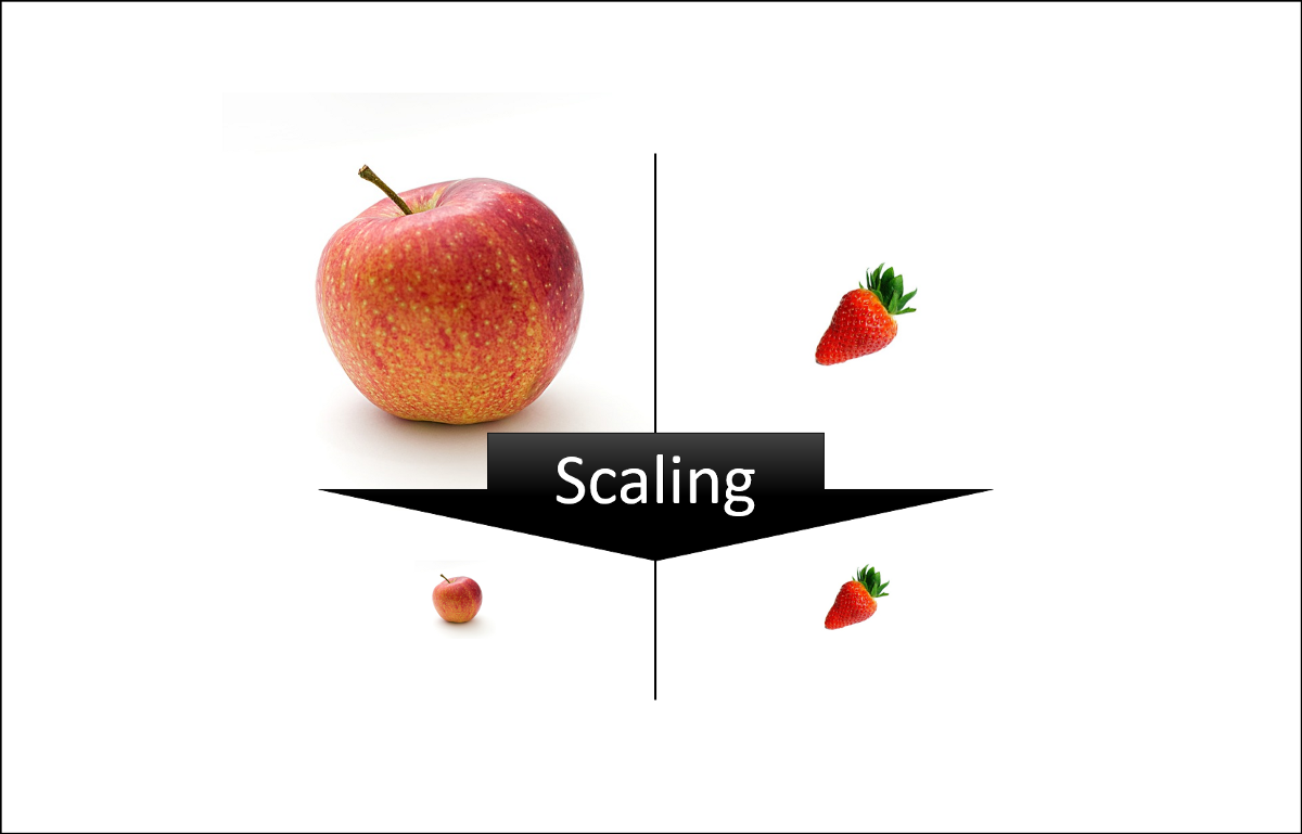
Feature Scaling
Feature Scaling is a technique to standardize the independent features present in the data in a fixed range.
Example, if we have weight of a person in a dataset with values in the range 15kg to 100kg, then feature scaling transforms all the values to the range 0 to 1 where 0 represents lowest weight and 1 represents highest weight instead of representing the weights in kgs.
Types of Feature Scaling:
1. Standardization
- Standard Scaler - (Z Score Normalization)
2. Normalization
- Min Max Scaling
- Max Absolute Scaling
- Mean Normalization
- Robust Scaling
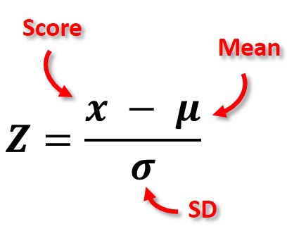
Standardization (Standard Scaler)
Standardization is a scaling technique where the values are centered around the mean with a unit standard deviation. This means that the mean of the attribute becomes zero and the resultant distribution has a unit standard deviation. Also known as Z Score Normalization.
Normalization
The goal of normalization is to change the values of numeric columns in the dataset to use a common scale, without distorting differences in the ranges of values or losing information.
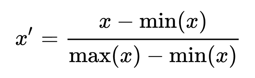
1. Min Max Scaling
The minimum value of that feature transformed into 0, the maximum value transformed into 1, and every other value gets transformed into a decimal between 0 and 1.
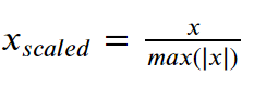
2. Max Absolute Scaling
maximal value of each feature in the training set will be 1. It does not shift/center the data, and thus does not destroy any sparsity.
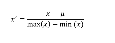
3. Mean Normalization
It is very similar to Min Max Scaling, just that we use mean to normalize the data. Removes the mean from the data and scales it into max and min values.
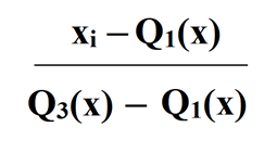
4. Robust Scaling
This Scaler removes the median and scales the data according to the quantile range (defaults to IQR: Interquartile Range). The IQR is the range between the 1st quartile (25th quantile) and the 3rd quartile (75th quantile).
The Big Question – Normalize or Standardize?
- Normalization is good to use when you know that the distribution of your data does not follow a Gaussian distribution. This can be useful in algorithms that do not assume any distribution of the data like K-Nearest Neighbors and Neural Networks.
- Standardization, on the other hand, can be helpful in cases where the data follows a Gaussian distribution. However, this does not have to be necessarily true. Also, unlike normalization, standardization does not have a bounding range. So, even if you have outliers in your data, they will not be affected by standardization.
What is Feature Engineering?
Feature Engineering is the process of extracting and organizing the important features from raw data in such a way that it fits the purpose of the machine learning model. It can be thought of as the art of selecting the important features and transforming them into refined and meaningful features that suit the needs of the model.
Eg: Creating a feature Area from length and breadth features in data.
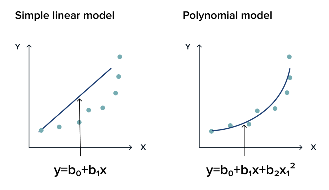
Why Polynomial Regression?
Suppose if we have non-linear data then Linear regression will not capable to draw a best-fit line and It fails in such conditions. consider the below diagram which has a non-linear relationship and you can see the Linear regression results on it, which does not perform well means which do not comes close to reality. Hence, we introduce polynomial regression to overcome this problem, which helps identify the curvilinear relationship between independent and dependent variables.
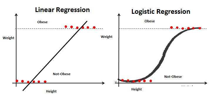
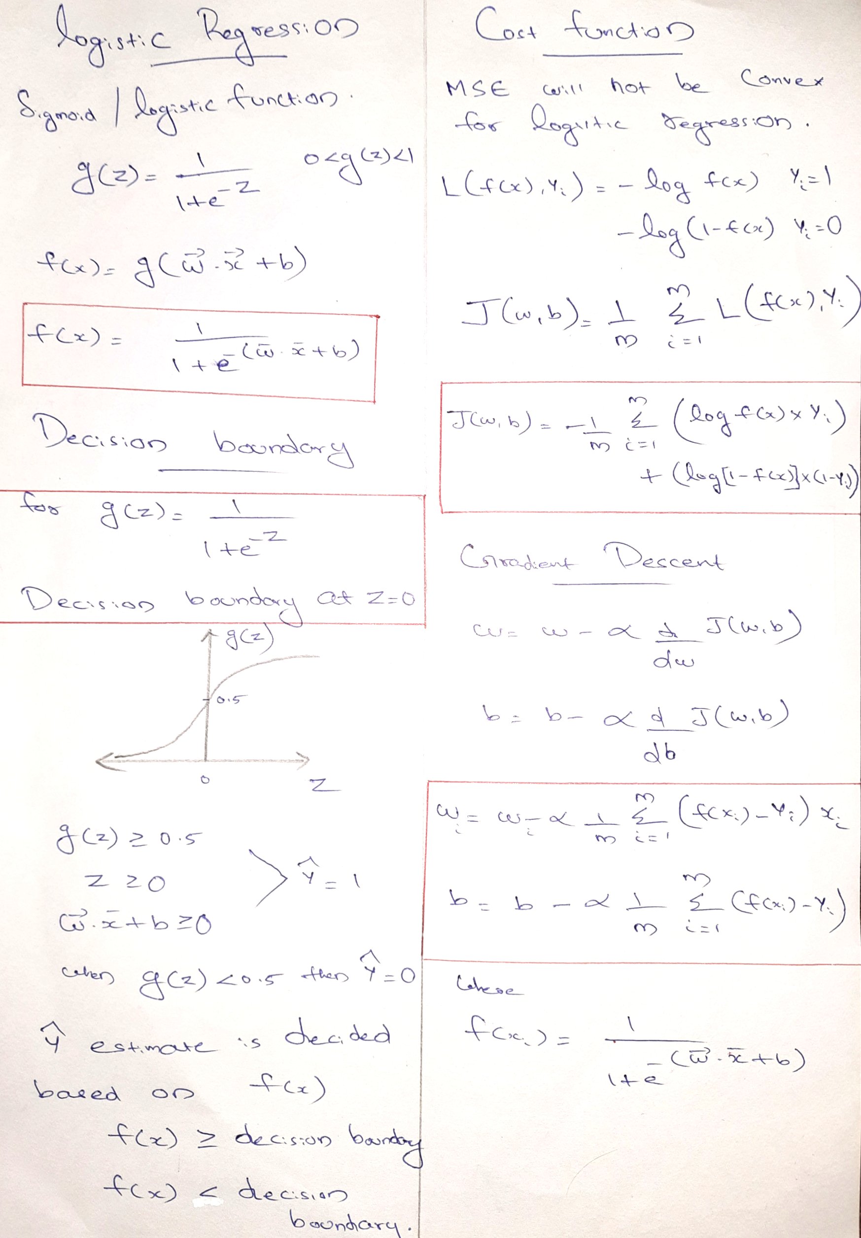
LOGISTIC REGRESSION
- Logistic regression is a predictive analysis of Probabilities for classification problems.
- It is used when our dependent variable has only 2 outputs.
- Eg: A person will survive this accident or not, The student will pass this exam or not.
Here we replace linear function with Logistic/Sigmoid Function
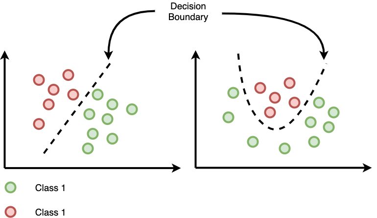
Decision Boundary – Logistic Regression
- The line or margin that separates the classes.
- Classification algorithms are all about finding the decision boundaries.
- It need not be straight line always.
- For a logistic function f(x), the g(z), where z = wx+b,
z = 0 gives the decision boundary. ie wx+b = 0
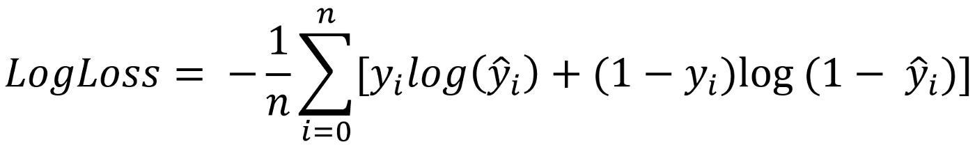
What is Log Loss?
Log-loss is indicative of how close the prediction probability is to the corresponding actual/true value (0 or 1 in case of binary classification).
- Lower log loss value means better prediction
- Higher log loss means worse prediction
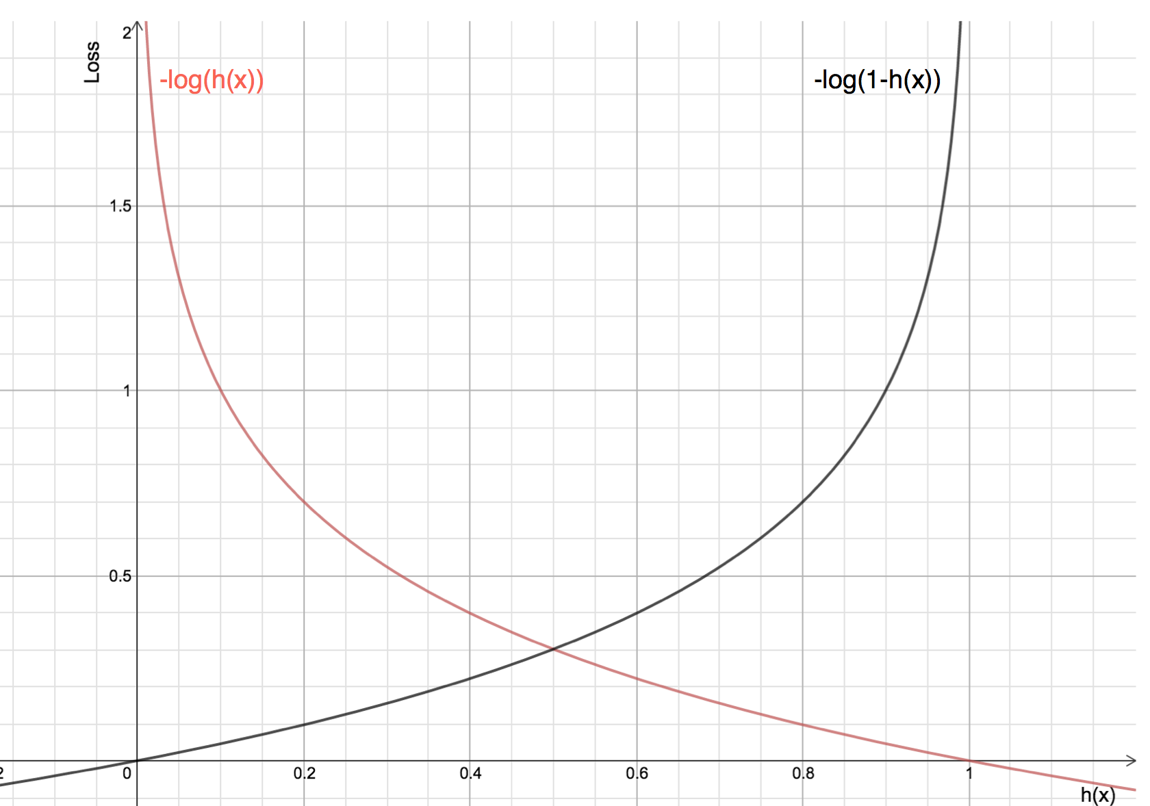
Equation of Log Loss Cost Function
- For Y = 0, Log Loss graph show low loss for y = 0 and high loss for y = 1
- For Y = 1, Log Loss graph show high loss for y = 0 and low loss for y = 1
Learning Curve, Vectorization, Feature Scaling all works same for Logistic Regression just like Linear Regression.
Overfitting and Underfitting in Machine Learning
Overfitting and Underfitting are the two main problems that occur in machine learning and degrade the performance of the machine learning models.
Before understanding the overfitting and underfitting, let's understand some basic term that will help to understand this topic well:
- Signal: It refers to the true underlying pattern of the data that helps the machine learning model to learn from the data.
- Noise: Noise is unnecessary and irrelevant data that reduces the performance of the model.
- Bias: It is the difference between the predicted values and the actual values. It is a prediction error in the model due to oversimplifying the machine learning algorithms.
- Variance: If the machine learning model performs well with the training dataset, but does not perform well with the test dataset, then variance occurs.
Overfitting
- Overfitting occurs when our machine learning model tries to cover all the data points.
- Model starts caching noise and inaccurate values present in the dataset, and all these factors reduce the efficiency and accuracy of the model.
- The overfitted model has low bias and high variance.
- The chances of overfitting increase as we provide more training to our model.
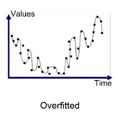
It may look efficient, but in reality, it is not so. Because the goal of the regression model to find the best fit line, but here we have not got any best fit, so, it will generate the prediction errors.
How to avoid the Overfitting:
Both overfitting and underfitting cause the degraded performance of the machine learning model. But the main cause is overfitting, so there are some ways by which we can reduce the occurrence of overfitting in our model.
- Cross-Validation
- Training with more data
- Ensembling (Technique that combines several base models to produce one optimal model)
- Removing features
- Early stopping the training
- Regularization (Reduce Size of Parameters)
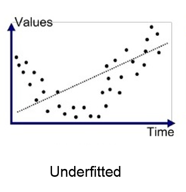
Underfitting
- In the case of underfitting, the model is not able to learn enough from the training data, and hence it reduces the accuracy and produces unreliable predictions.
- Underfitted model has high bias and low variance.
How to avoid Underfitting:
- By increasing the training time of the model.
- By increasing the number of features.
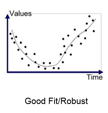
Goodness of Fit
The model with a good fit is between the underfitted and overfitted model, and ideally, it makes predictions with 0 errors, but in practice, it is difficult to achieve it.
As when we train our model for a time, the errors in the training data go down, and the same happens with test data. But if we train the model for a long duration, then the performance of the model may decrease due to the overfitting, as the model also learn the noise present in the dataset. The errors in the test dataset start increasing, so the point, just before the raising of errors, is the good point, and we can stop here for achieving a good model.
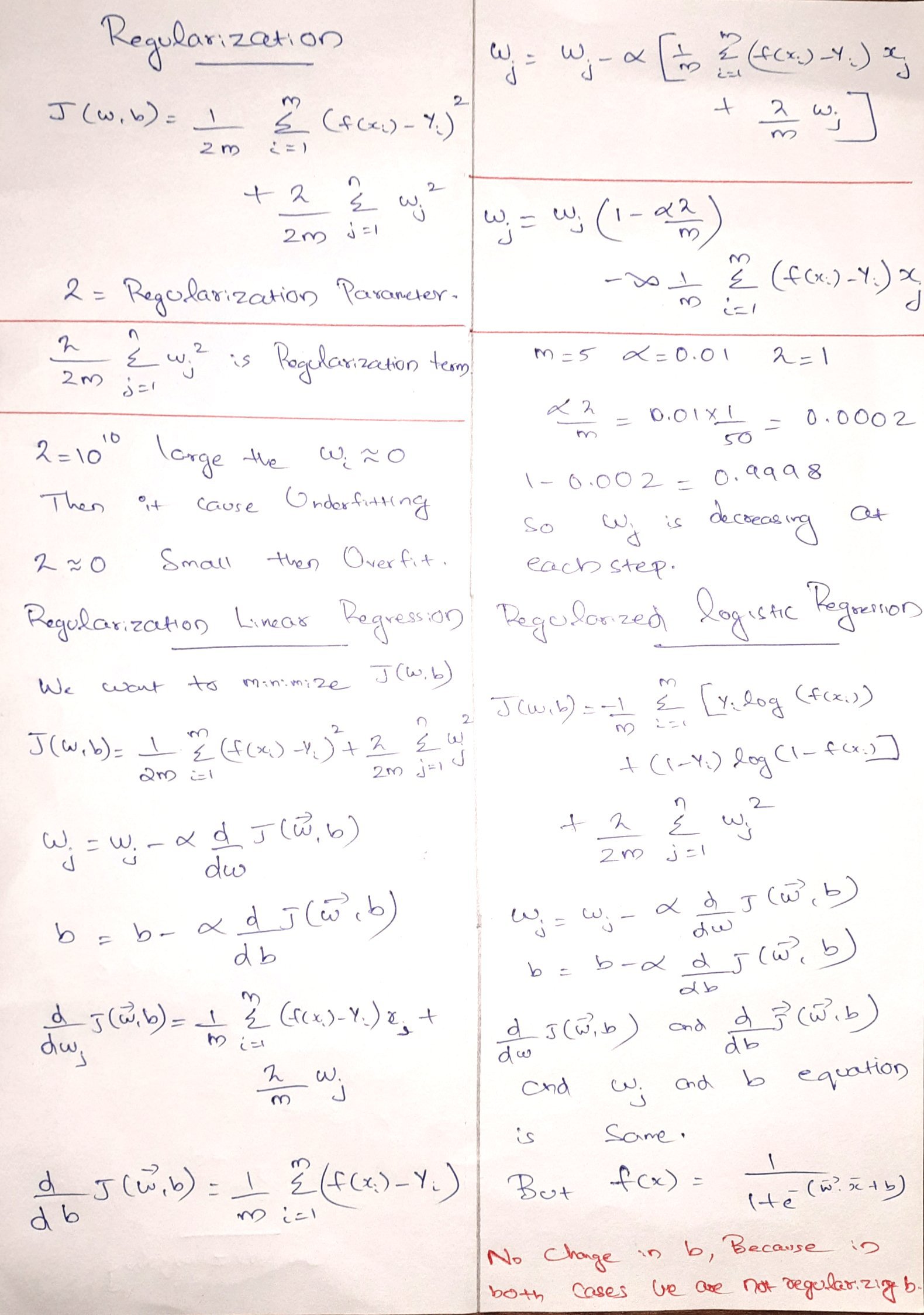
REGULARIZATION
We mainly regularizes or reduces the coefficient of features toward zero. In simple words, "In regularization technique, we reduce the magnitude of the features by keeping the same number of features."
Types of Regularization Techniques
There are two main types of regularization techniques: L1(Lasso) and L2( Ridge) regularization
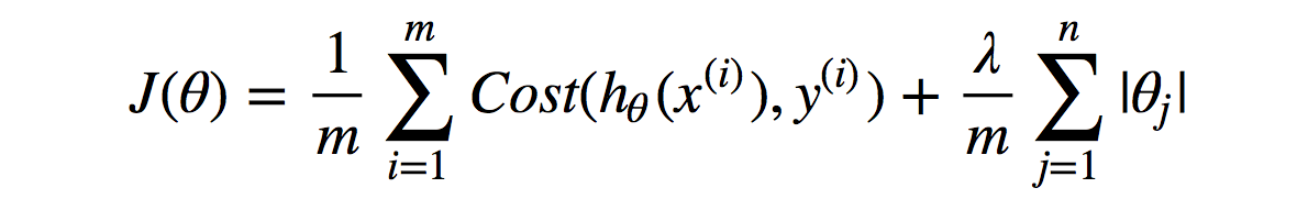
1) Lasso Regularization (L1 Regularization)
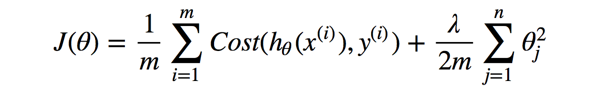
In L1 you add information to model equation to be the absolute sum of theta vector (θ) multiply by the regularization parameter (λ) which could be any large number over size of data (m), where (n) is the number of features.
2) Ridge Regularization (L2 Regularization)
In L2, you add the information to model equation to be the sum of vector (θ) squared multiplied by the regularization parameter (λ) which can be any big number over size of data (m), which (n) is a number of features.
Advanced Learning Algorithms - Course 2
NEURAL NETWORKS
- Learning Algorithms that mimic the Human Brain.
- Speech Recognition, Computer Vision, NLP, Climate Change, Medical Image Detection, Product Recommendation.
- Just like human neuron, neural networks use many neurons to receive input and gives an output to next layer of network.
- As amount of data increased the performance of neural networks also increased.
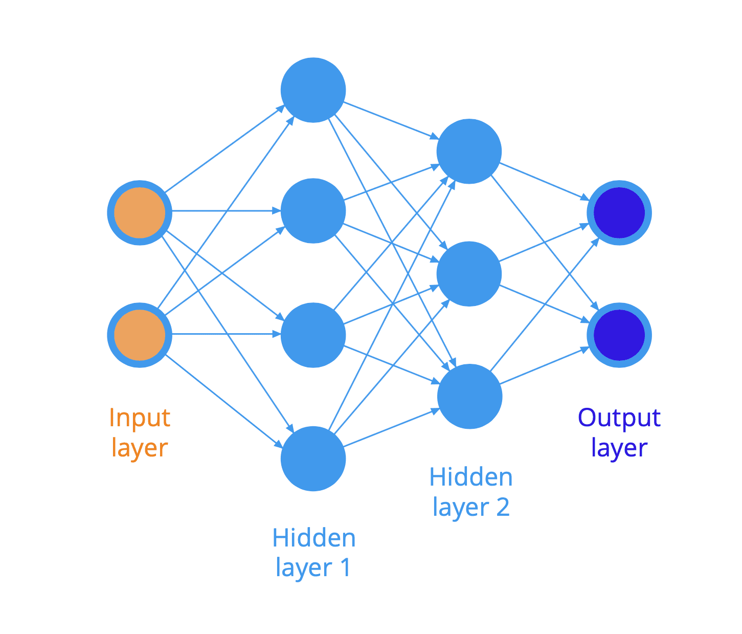
- Layer is a grouping of neurons, which take input of similar features and output a few numbers together.
- Layer can have single or multiple neurons.
- If the layer is first, it is called Input Layer
- If the layer is last it is called Output Layer
- If the layer in middle, it is called Hidden Layer
- Each neurons have access to all other neurons in next layer.
Activations (a)
- Refers to the degree of high output value of neuron, given to the next neurons.
- Neural Networks learn it’s own features. No need of manual Feature Engineering.
Demand Prediction of a Shirt?
- affordability, awareness, perceived quality are activations of each neurons.
- It is basically a Logistic Regression, trying to learn much by it’s own.
- activation, a = g(z) = 1 / ( 1 + e ^ -z)
- Number of layers and neurons are called Neural Network Architecture.
- Multi-layer perception is also known as MLP. It is fully connected dense layers.
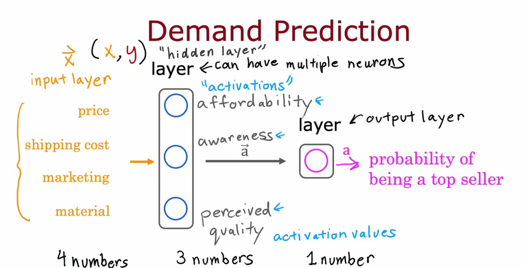
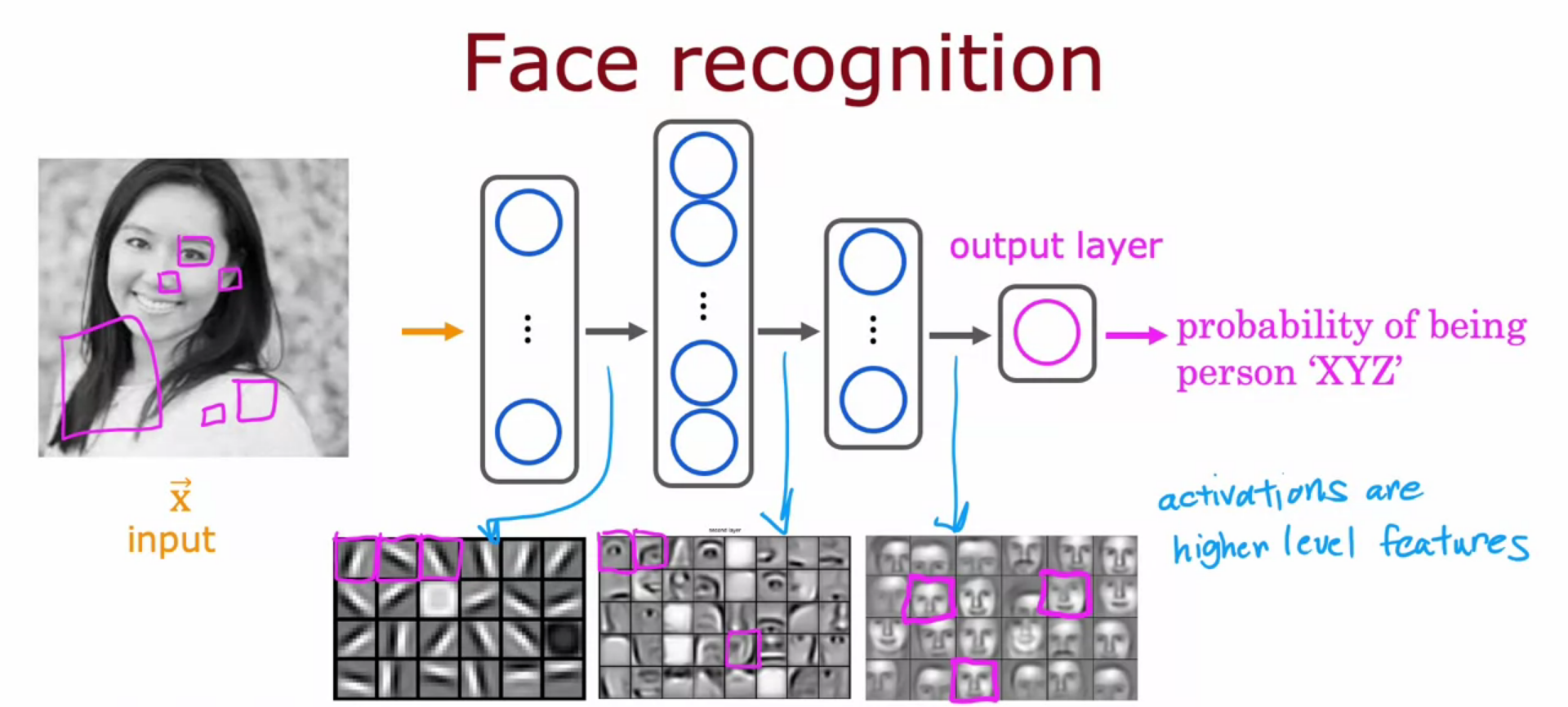
Image Recognition
- For a 1000 * 1000 pixel image we have a vector of 1 million elements.
- We build a neural network by providing that as an input.
- In each hidden layer they are improving the recognition all by itself.
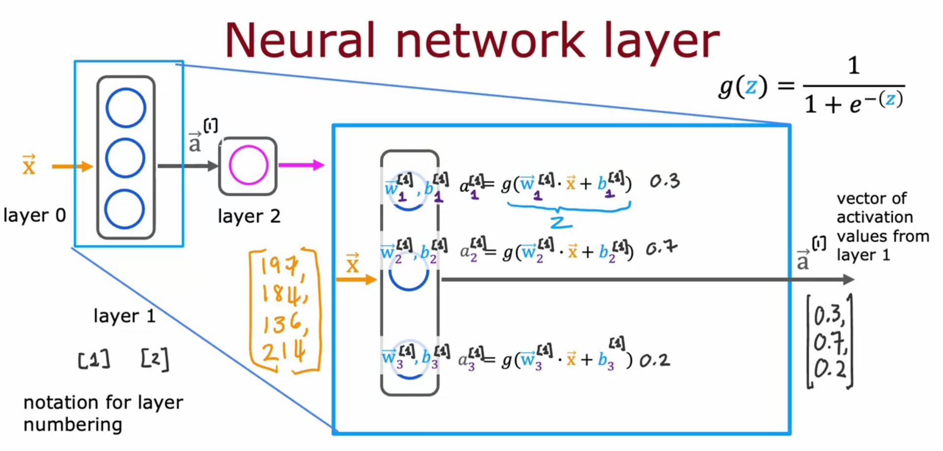
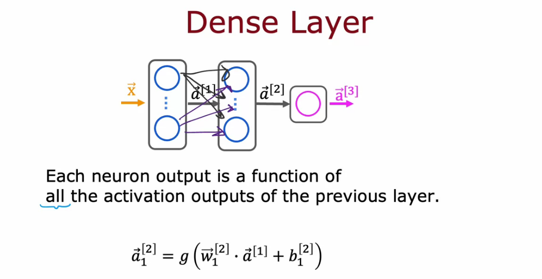
Neural Network Layer
- Each neuron is implementing the activation of Logistic Regression.
- Super script square bracket 1 means quantity that is associated with Neural Network 1 and so on.
- Input of layer 2 is the output of layer 1. It will be a set of vectors.
- Every layer input a vector of numbers and output a vector of numbers

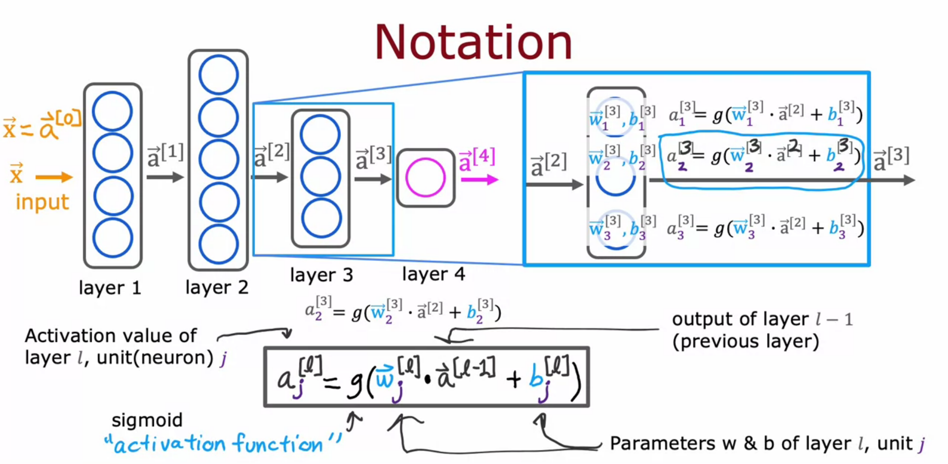
Complex Neural Network
- aj[l] where j is the neuron/unit and l is the layer
- g(w.a+b) is the activation function(sigmoid function etc can be used here)
- input layer is a[0]
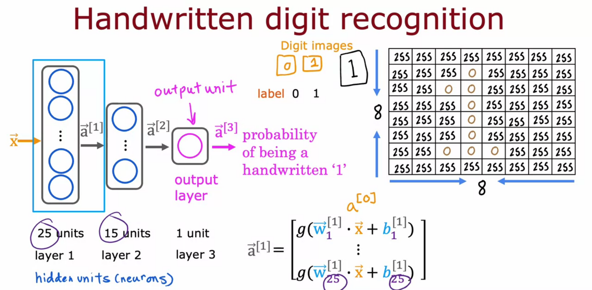
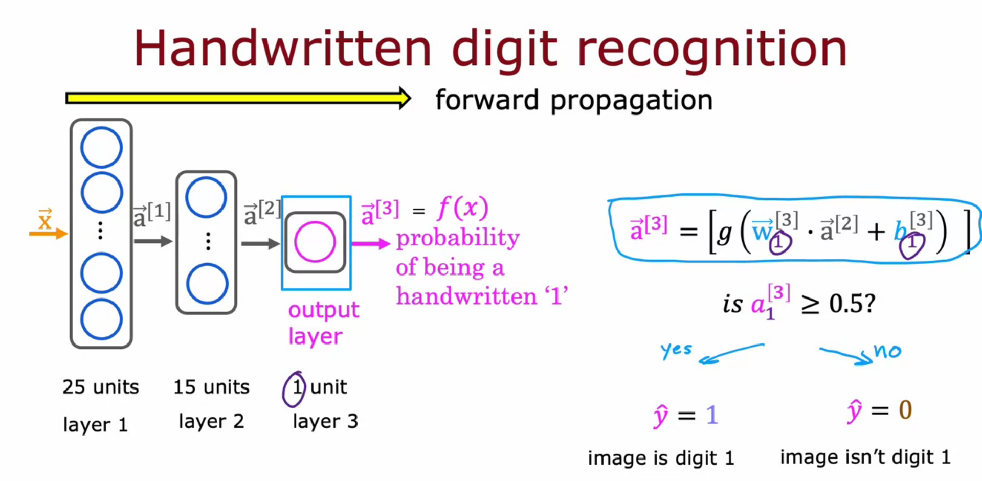
Inference/Make Prediction (Handwritten Digit Recognition)
Forward Propagation
- If activation computation goes from left to right it is called, Forward Propagation.
Calculation of first layer vector
Calculation of second layer vector
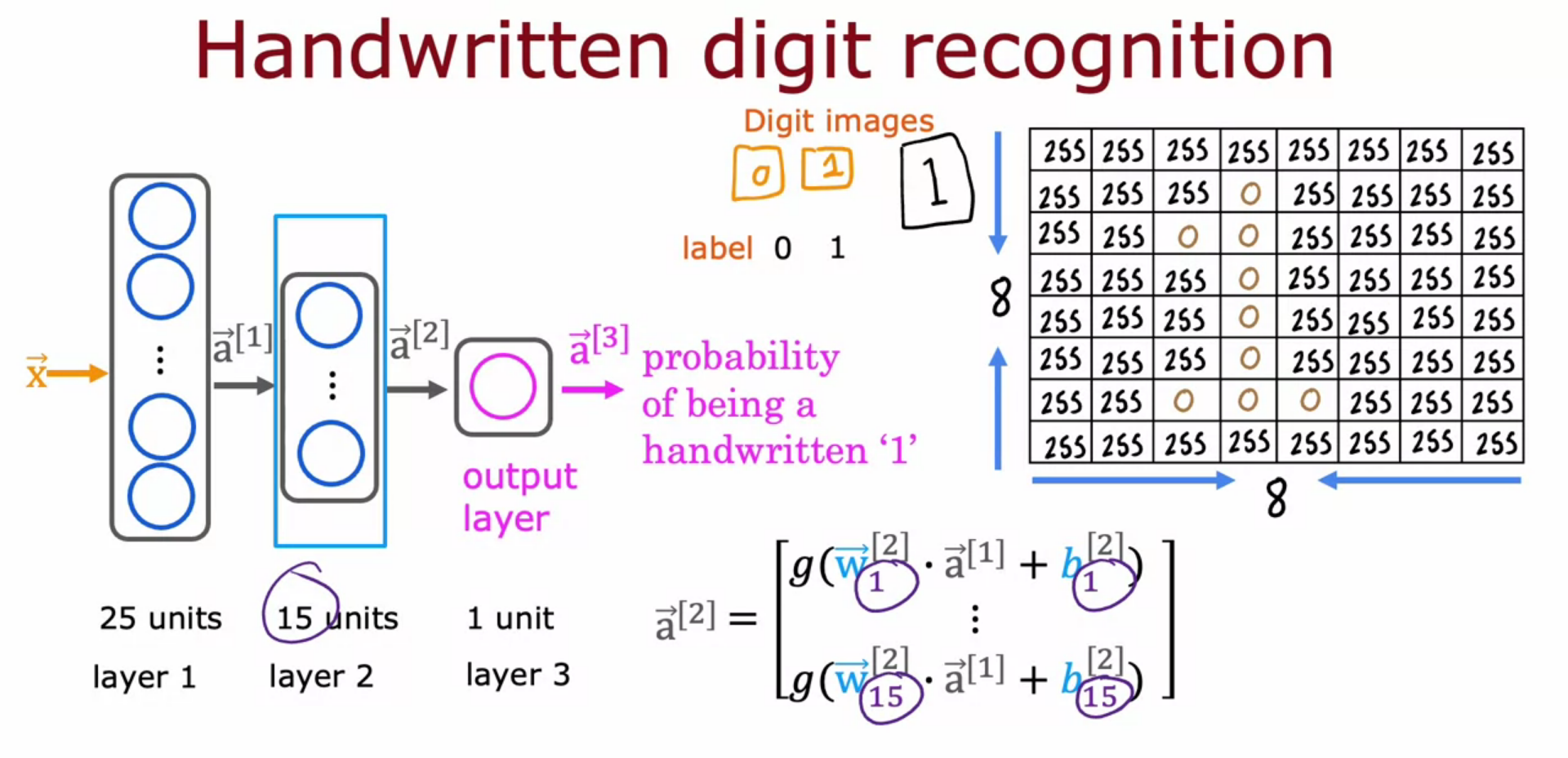
Calculation of last layer vector
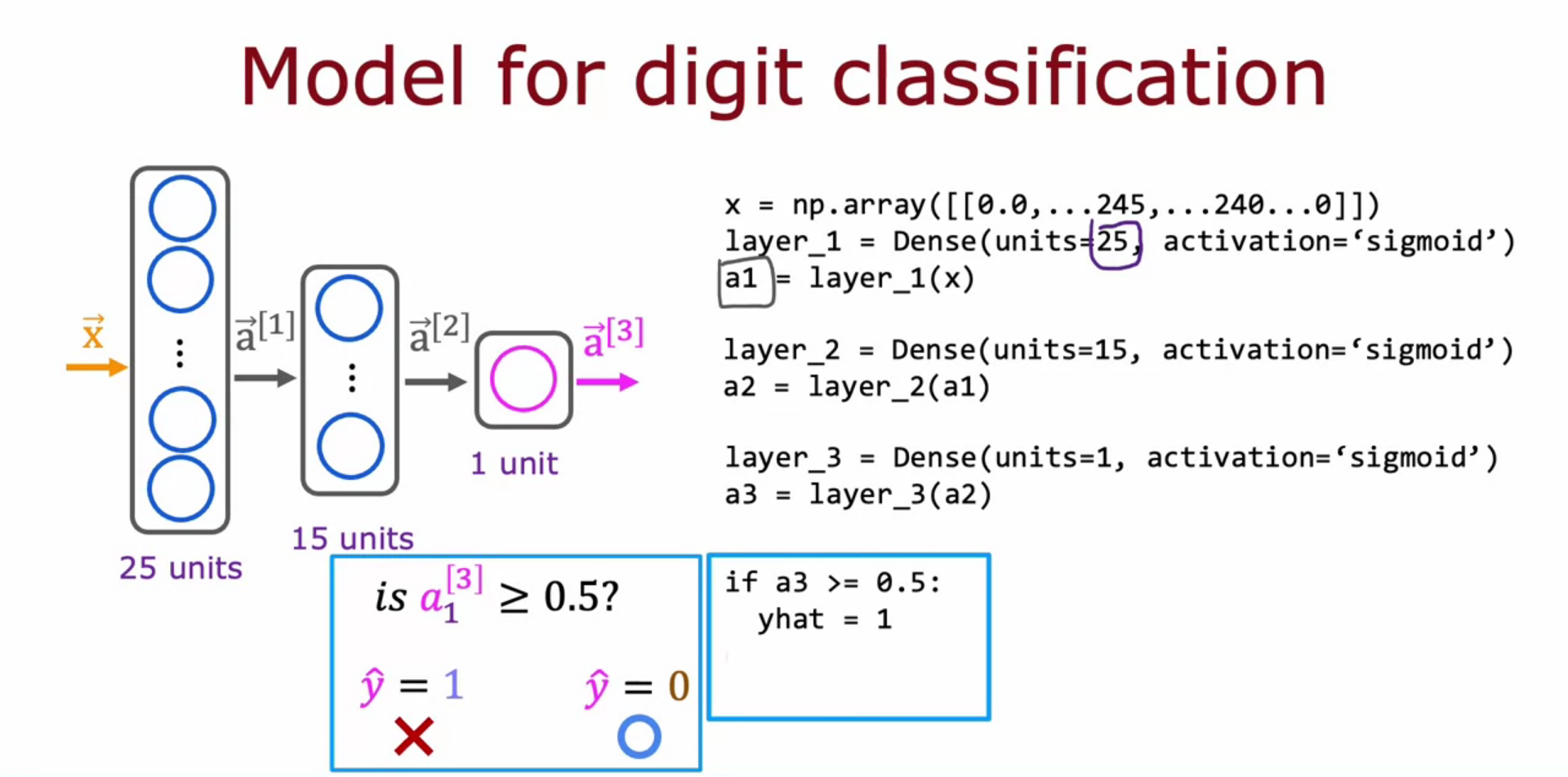
Tensorflow Implementation
- building a layer of NN in tensorflow below for handwritten digit 0/1 classification
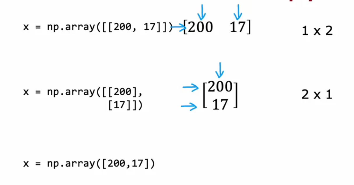
Data in Tensorflow
- Inconsistency between data in Numpy and Tensorflow
- Numpy we used 1D vector, np.array( [ 200, 18 ] )
- Tensorflow uses matrices, np.array( [ [ 200, 18] ] )
- Representing in Matrix instead of 1D array make tensorflow run faster.
- Tensor is something like matrix
Activation of Vector
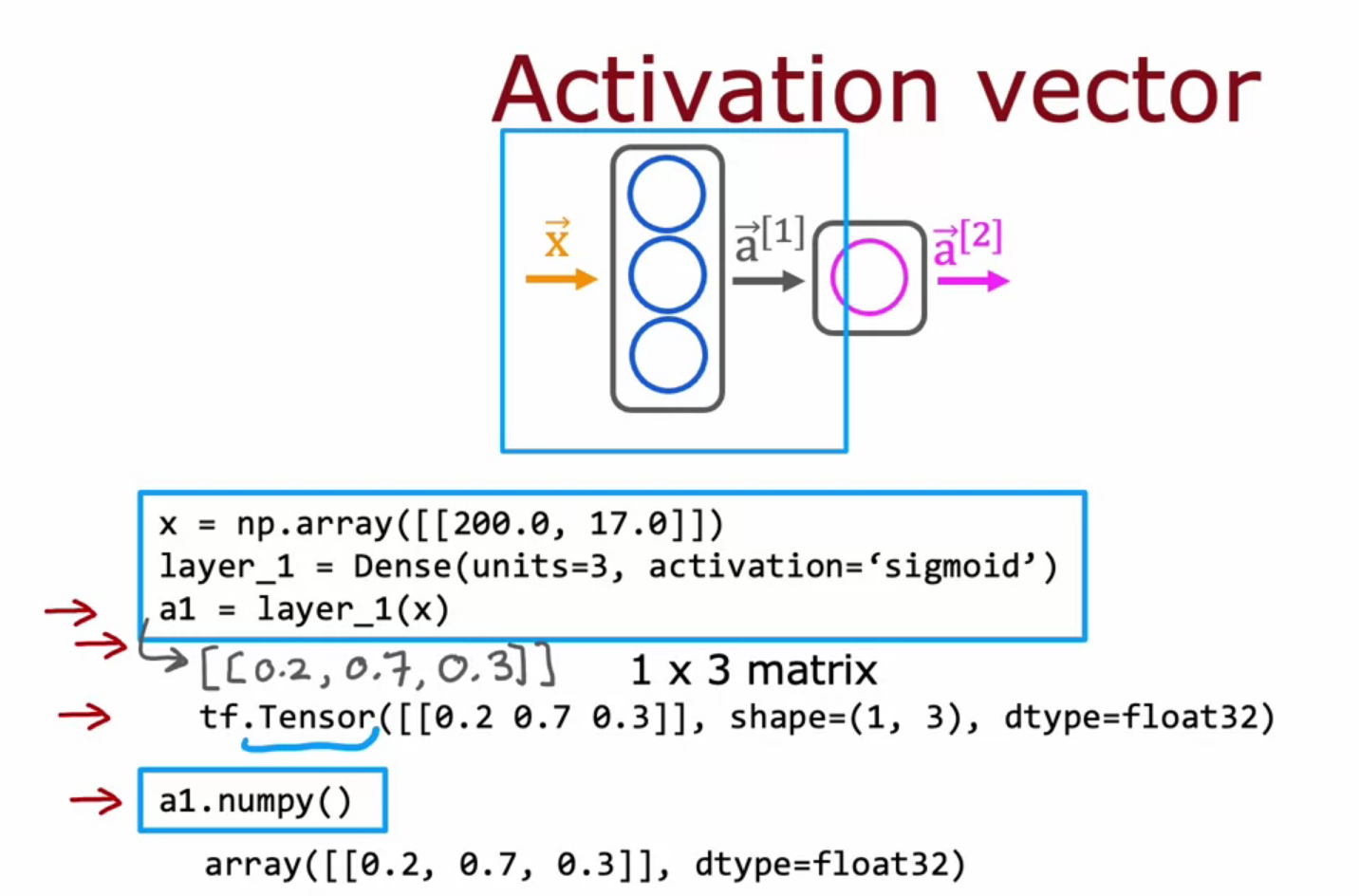
Building a Neural Network in Tensorflow
Digit Classification Model
import tensorflow as tf
layer_1 = Dense( units=25, activation=”sigmoid” )
layer_2 = Dense( units=15, activation=”sigmoid” )
layer_3 = Dense( units=1, activation=”sigmoid” )

model = Sequential ( [ layer_1, layer_2, layer_3 ] )

x = np.array( [ [ 0….., 245, ….., 17 ],
								[ 0….., 200, ….., 184 ]  ] )
y = np.array( [ 1, 0 ] )

model.compile(………………)
model.fit( x, y )
model.predict( new_x )
Forward Prop in Single Layer (Major Parts)
import tensorflow as tf
from tensorflow.keras.layers import Dense
from tensorflow.keras.models import Sequential

model = Sequential(
    [
        tf.keras.Input(shape=(2,)),
        Dense(3, activation='sigmoid', name = 'layer1'),
        Dense(1, activation='sigmoid', name = 'layer2')
     ]
)

model.compile(
    loss = tf.keras.losses.BinaryCrossentropy(),
    optimizer = tf.keras.optimizers.Adam(learning_rate=0.01),
)

model.fit(
    Xt,Yt,
    epochs=10,
)
General Implementation of Forward Prop in Single Layer
- Uppercase for Matrix
- Lowercase for Vectors and Scalers
def my_dense(a_in, W, b, g):
"""
Computes dense layer
Args:
a_in (ndarray (n, )) : Data, 1 example
W (ndarray (n,j)) : Weight matrix, n features per unit, j units
b (ndarray (j, )) : bias vector, j units
g activation function (e.g. sigmoid, relu..)
Returns
a_out (ndarray (j,)) : j units|
"""
units = W.shape[1]
a_out = np.zeros(units)
for j in range(units):
w = W[:,j]
z = np.dot(w, a_in) + b[j]
a_out[j] = g(z)
return(a_out)
def my_sequential(x, W1, b1, W2, b2):
a1 = my_dense(x, W1, b1, sigmoid)
a2 = my_dense(a1, W2, b2, sigmoid)
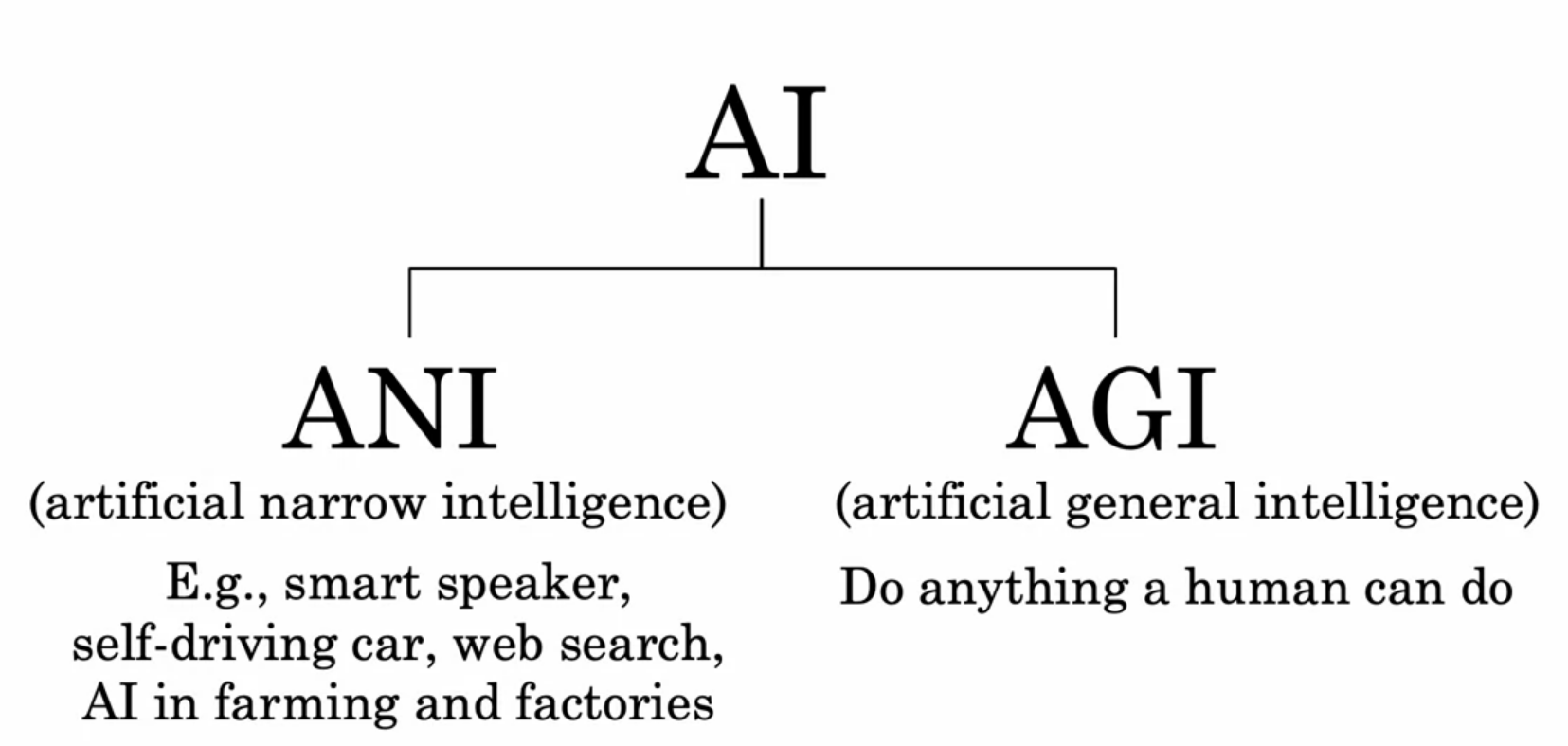
return(a2)Artificial General Intelligence - AGI

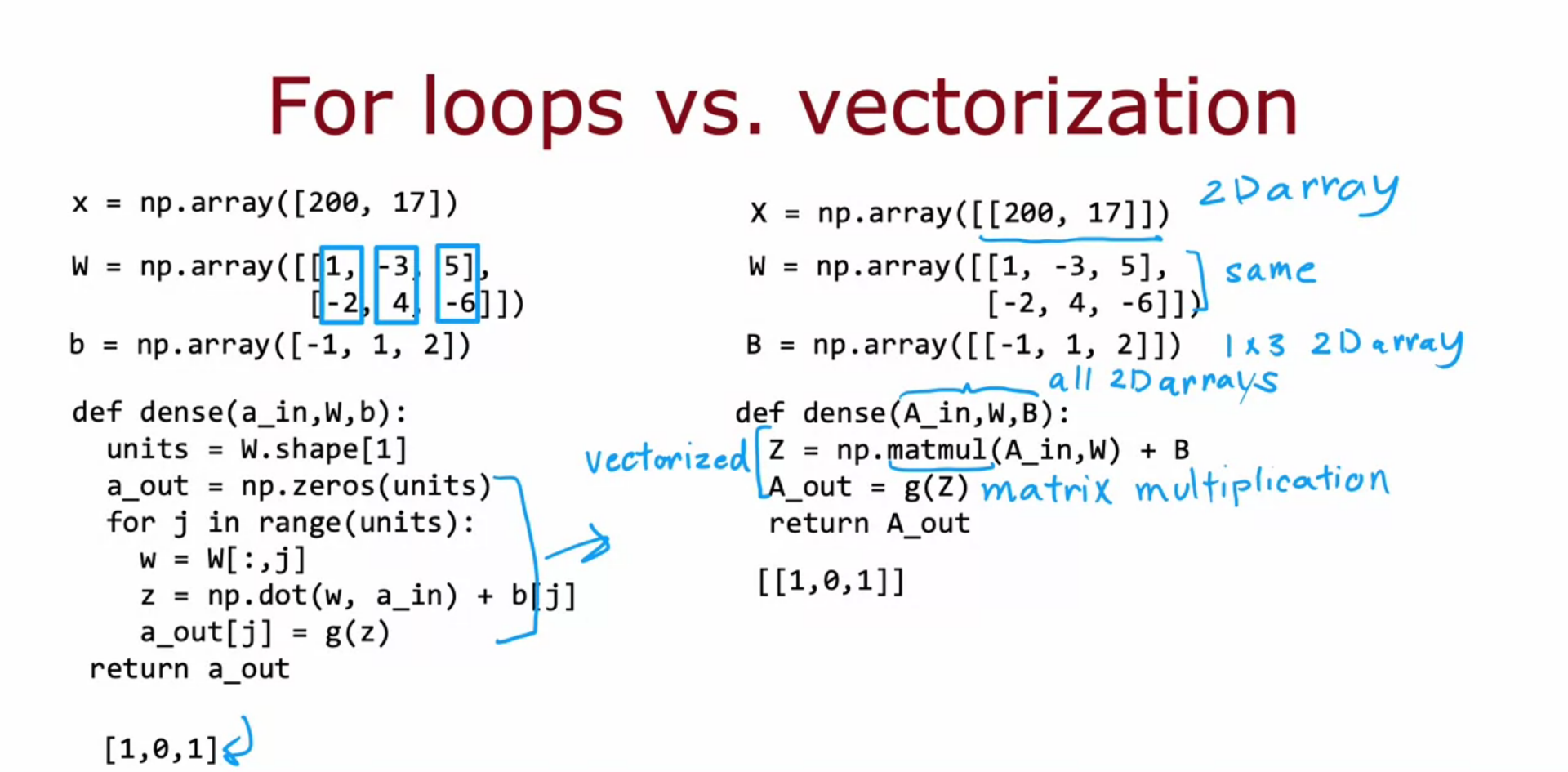
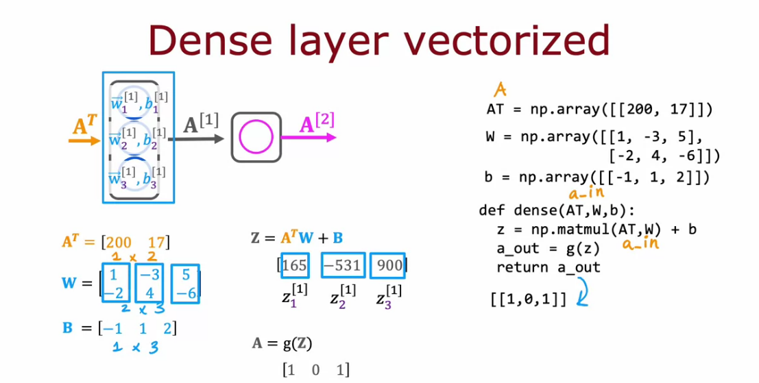
Vectorization
- Matrix Multiplication in Neural Networks using Parallel Computer Hardware
- Matrix Multiplication Replaces For Loops in speed comparison
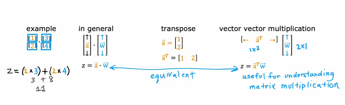
Dot Product to Matrix Multiplication using Transpose
- a . w = a1*w1 + a2+w2 + ………. + an*wn
- a . w = a^T * w
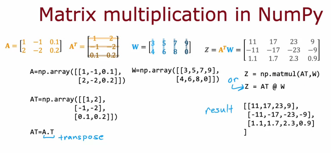
Matrix Multiplication in Neural Networks
- Dot Product of vectors that have same length
- Matrix Multiplication is valid if col of matrix 1 = row of matrix 2
- Output will have row of matrix 1 and col of matrix 2
In code for numpy array and vectors
Dense Layer Vectorized
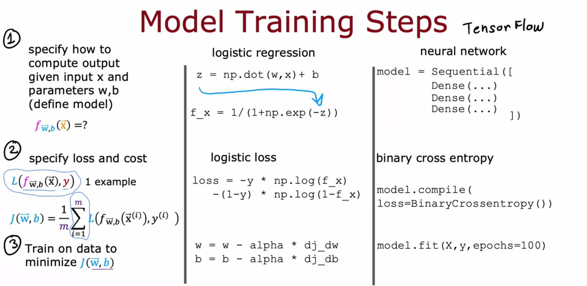
Tensorflow Training
- epoch is how many steps, the learning algorithm like gradient descent should run.
- BinaryCrossentropy is log loss function for logistic regression in classification problem
- if we have regression problem, use MeanSquaredError()
- loss = tf.keras.losses.MeanSquaredError()
- Derivatives of gradient descent has been calculated using backpropagation handled by model.fit
import tensorflow as tf
from tensorflow.keras.layers import Dense
from tensorflow.keras.models import Sequential

model = Sequential(
    [
        tf.keras.Input(shape=(2,)),
        Dense(3, activation='sigmoid', name = 'layer1'),
        Dense(1, activation='sigmoid', name = 'layer2')
     ]
)

model.compile(
    loss = tf.keras.losses.BinaryCrossentropy(),
    optimizer = tf.keras.optimizers.Adam(learning_rate=0.01),
)

model.fit(
    Xt,Yt,
    epochs=10,
)


Activation Function Alternatives
- awareness can not be binary, It better to use like like non negative number from zero to large number
- So best activation here is ReLU, Rectifier Linear Unit
- g( z ) = max( 0, z )
- ReLU is common choice of training neural networks and now used more than Sigmoid
- ReLU is faster
- ReLU is flat in one side, and Sigmoid flat on both sides. So gradient descent perform faster in ReLU
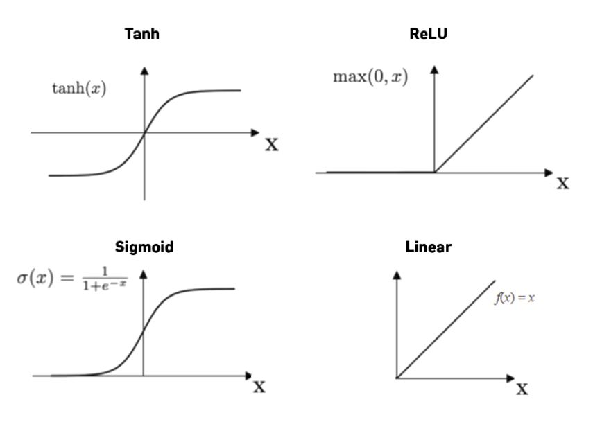
Choose Activation Function
For Output Layer
- Binary Classification - Sigmoid
- Regression - Linear
- Regression Positive Only - ReLU
For Hidden Layer
- ReLU as standard activation
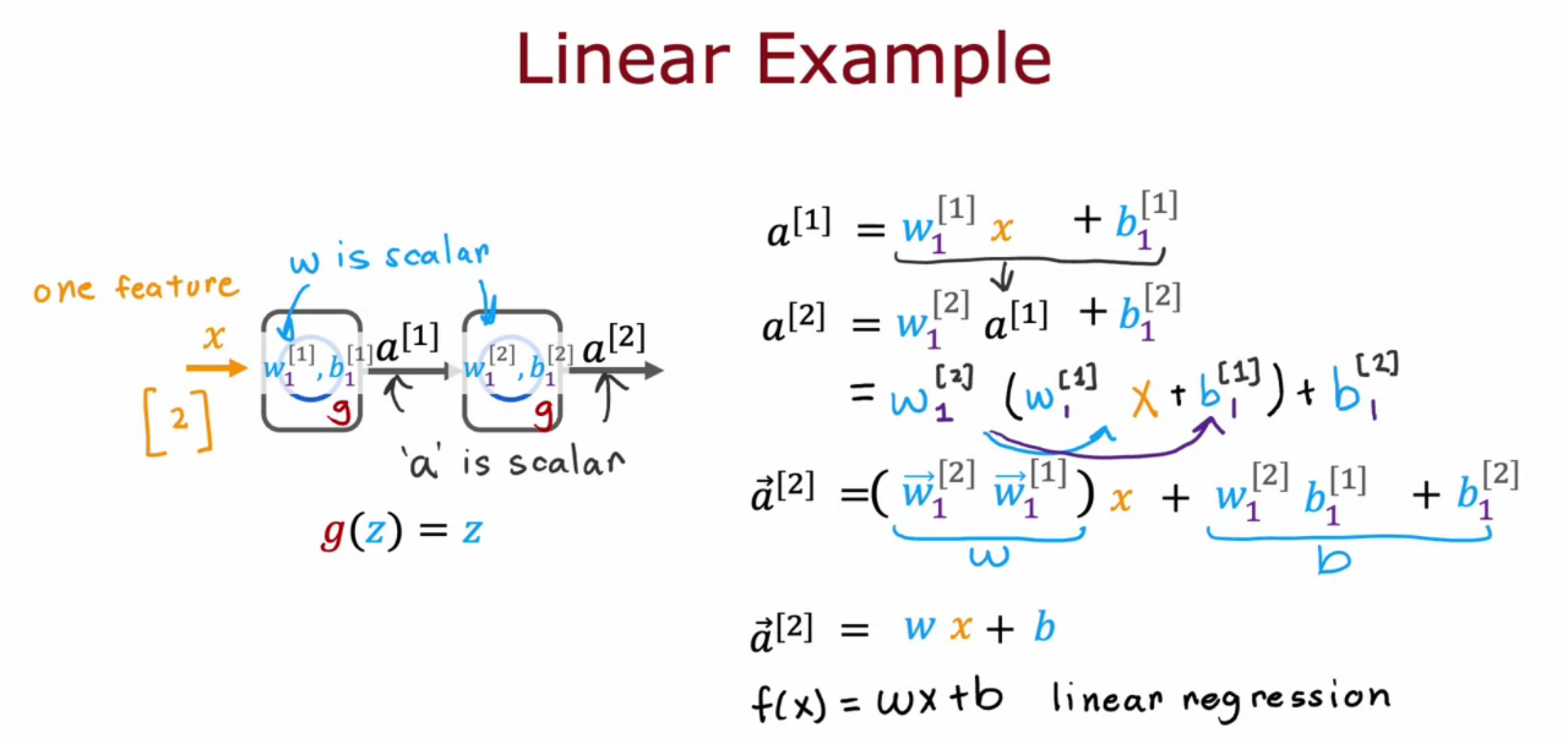
Why do we need activation functions?
- If we use linear activation function across all the neurons the neural network is no different from Linear Regression.
- If we use linear in hidden and sigmoid in output it is similar to logistic regression.
- Don’t use linear in hidden layers. Use ReLU
- We wont be able to fit anything complex

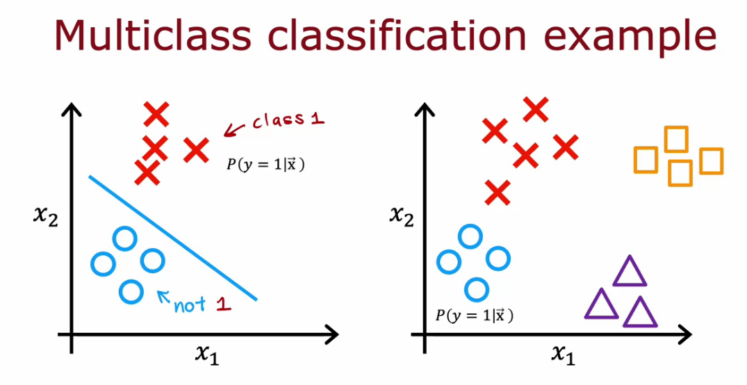
Multiclass Classification
- classification with more than 2 class is called multiclass classification
- Identifying a number is multiclass since we want to classify 10 number classes (MNIST)
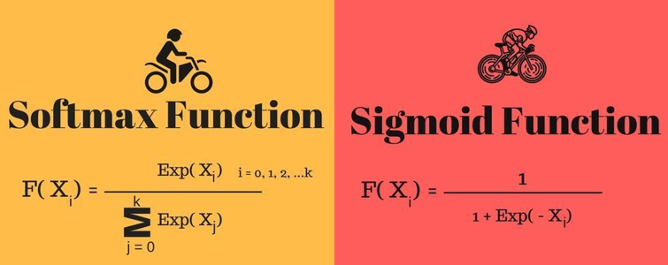
- for n = 2 softmax is basically logistic regression

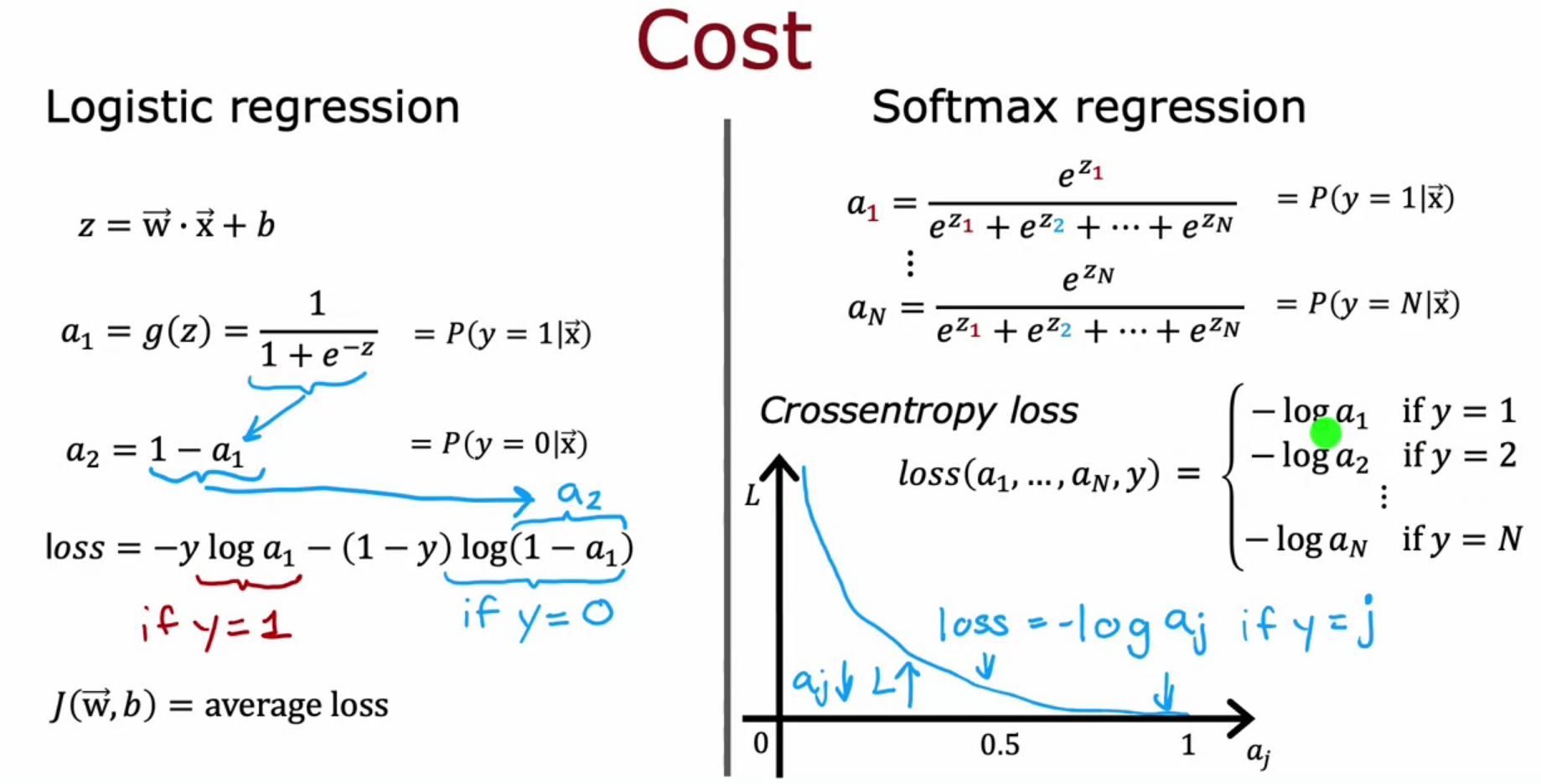
Cost Function of Softmax
- Cross entropy loss - if loss value is 1 smaller the loss.
- Cross entropy loss - if loss value is 0 larger the loss.
- Sigmoid - BinaryCrossEntropy
- Softmax - SparseCategoricalCrossEntropy


Don’t use the above way of code for implementation. We can use alternative efficient method.
Improved Implementation of Softmax
x1 = 2.0 / 10000
0.00020000000000

x2 = (1 + 1/10000) - (1 - 1/10000)
0.000199999999978

# due to memory constraints in computer rounding happens.
# inorder to avoid/reduce rounding up in softmax we can use other implementation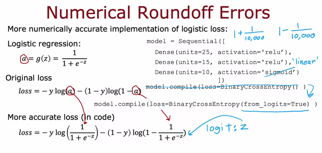


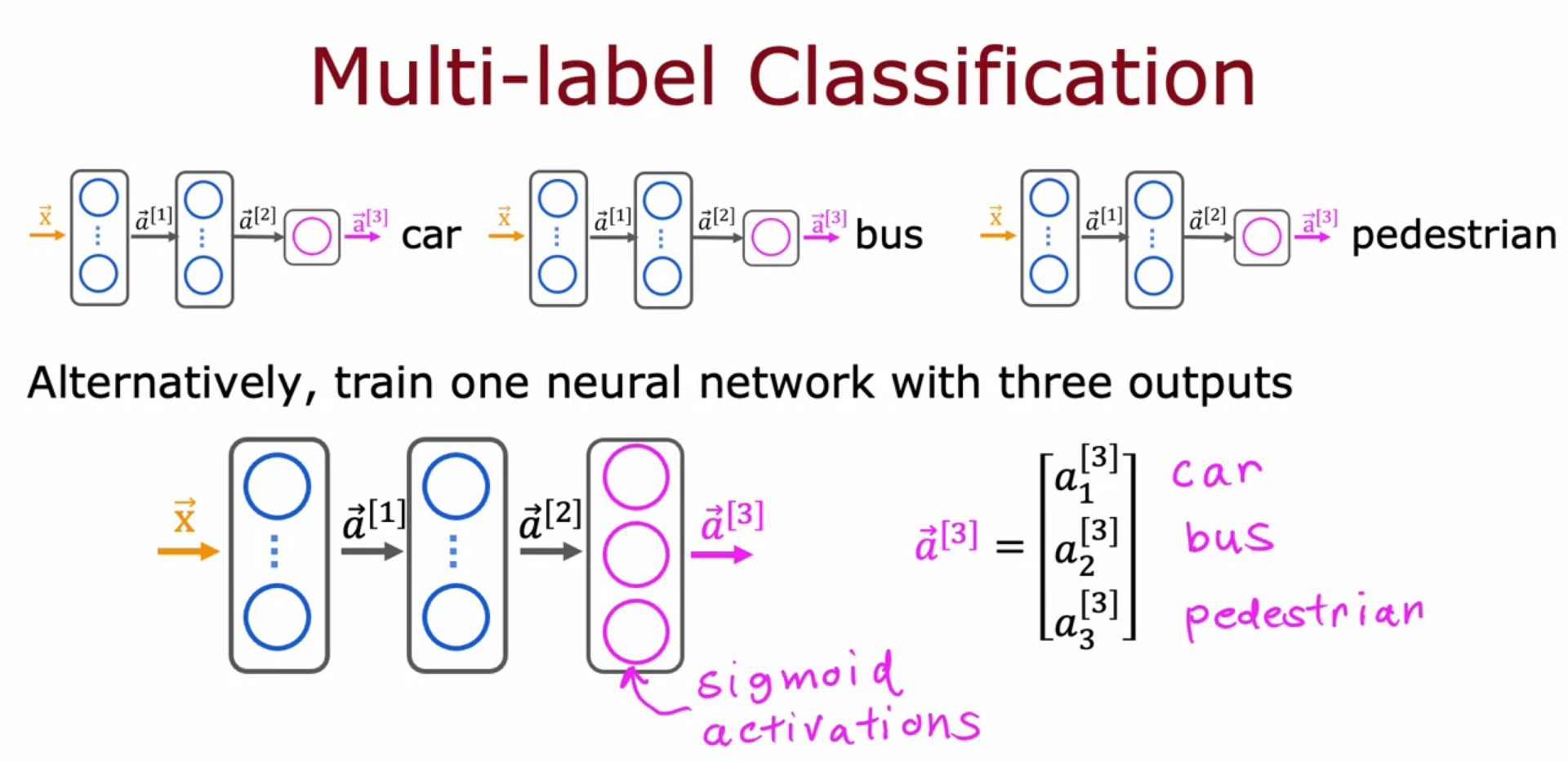
Multi Label Classification
- In single output there are multiple class, like returning a vector of possibility
- For self driving car it have multiple labels like is there a car? is there a bus? is there a man?
- It output result as [ 1, 0, 1 ]
- We cannot make different NN for each we want it in single NN
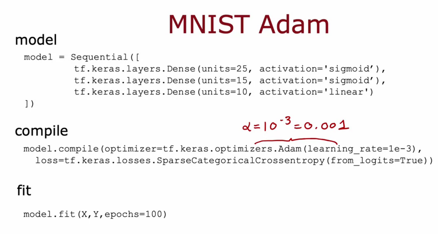
Adam - Adaptive Moment Estimation
- Adam Optimizer is a alternative for Gradient Descent
- It is faster than GD
- learning rate is not a constant one but multiple learning rate is used
- different Alpha should be tried like so small and large even after using 0.001
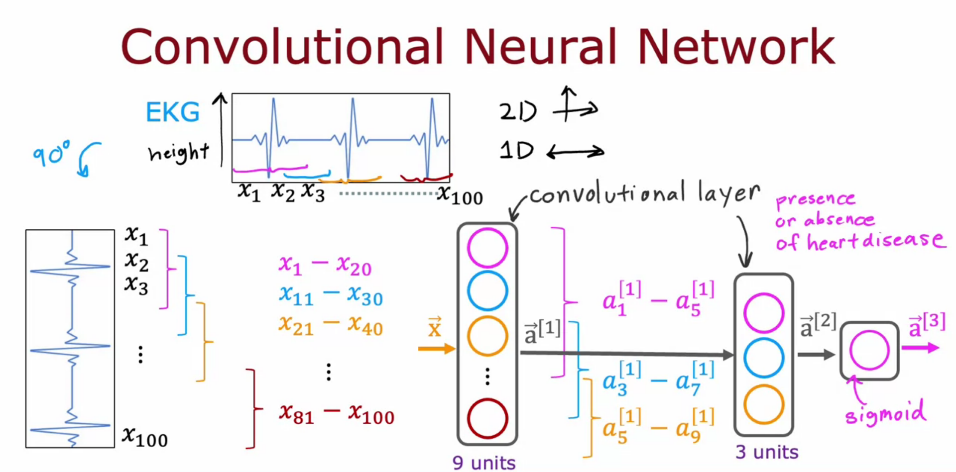
Convolutional Neural Network - CNN
- It is a layer alternative for Dense Layer
- Hidden layer in CNN can use a set or part for creating a NN (MNIST)
- each neuron only look at part of the previous layer’s input
- need less training data
- So due to this it can be fast
- we can avoid overfitting
Debugging a learning algorithm
- Get more training data
- try small set of features
- try large set of features
- try adding polynomial features
- try decreasing and increasing learning rate and lambda (regularization parameter)
- we can use different diagnostic systems
Evaluating your Model
- Split the data training and testing.
- we can find training error and testing error
- cost function should be minimized
- MSE for Linear Regression
- Log Loss for Logistic Regression - Classification
- For classification problem we can find what percentage of training and test set model which has predicted false, which is better than log loss
- we can use polynomial regression and test the data for various degree of polynomial
- But to improve testing we can split data into training, cross validation set and test set
- Even for NN we can use this type of model selection
- Then we can find the cost function for each set
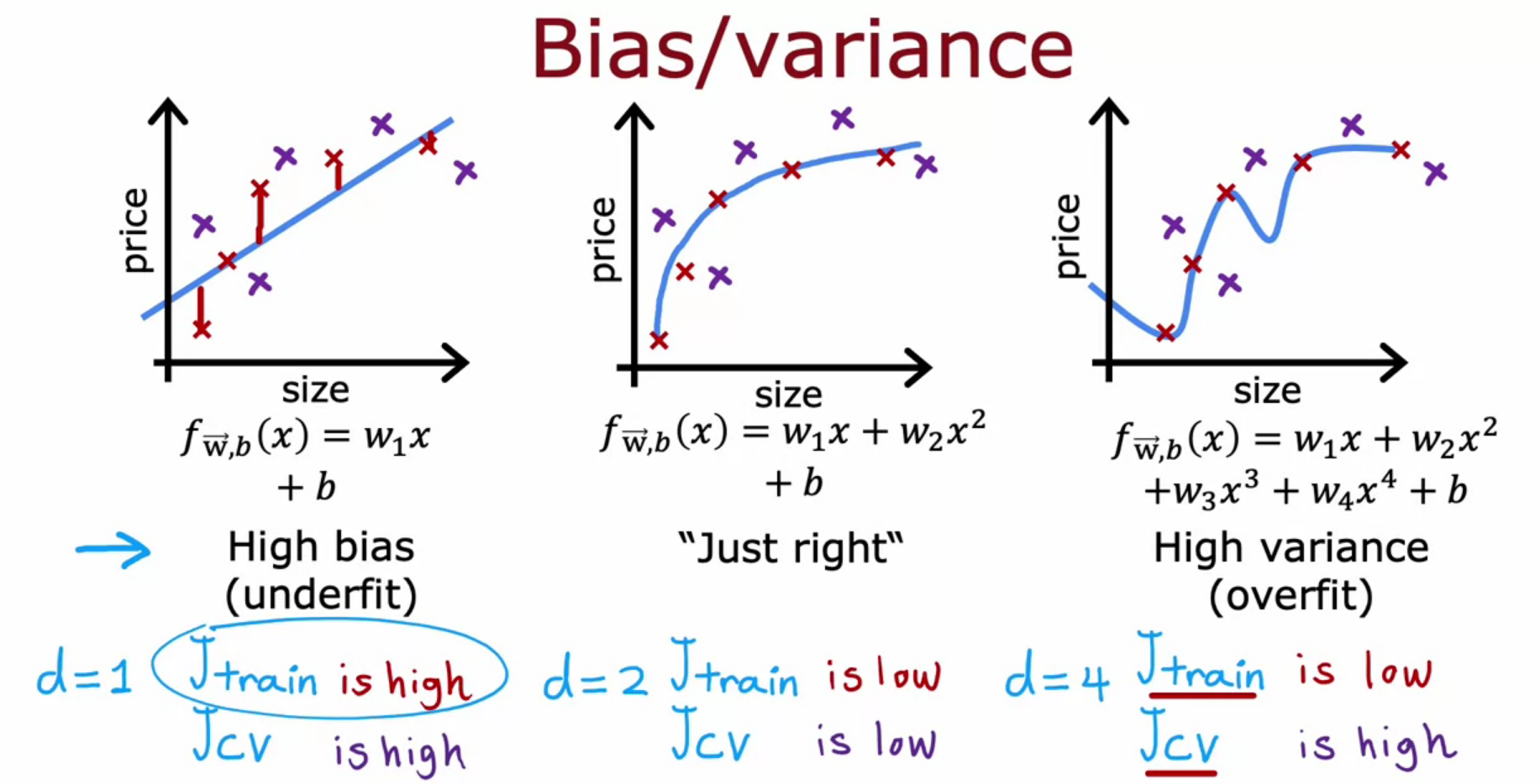
Bias and Variance - Model Complexity or High Degree Polynomial
- We need low bias and low variance
- Bias - Difference between actual and predicted value
- Variance - Perform well on training set and worse on testing set
- degree of polynomial should not be small or large. It should be intermediate

Regularization - Bias and Variance
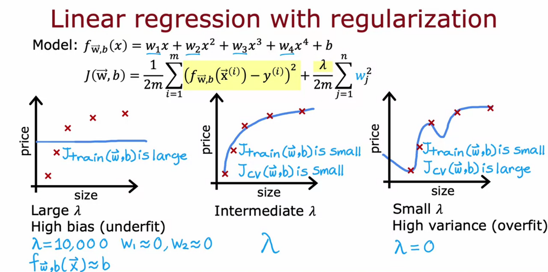

- Underfit - low Poly degree, high lambda (regularization parameter)
- Overfit - High Poly degree, Low lambda (regularization parameter)
- Intermediate lambda and Poly degree is best
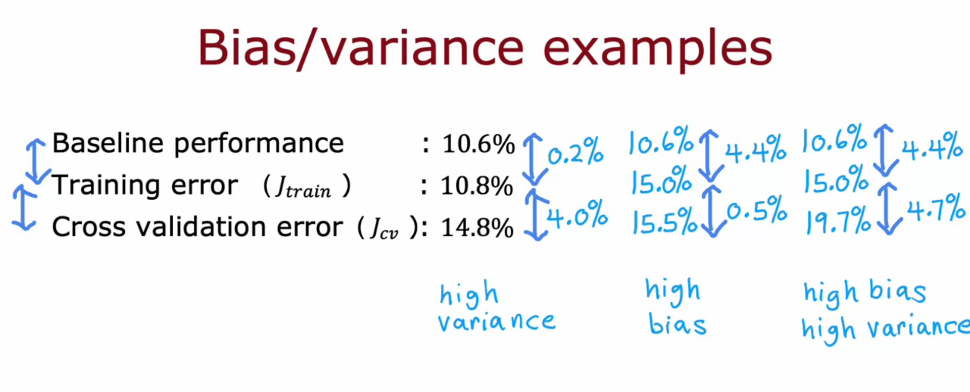
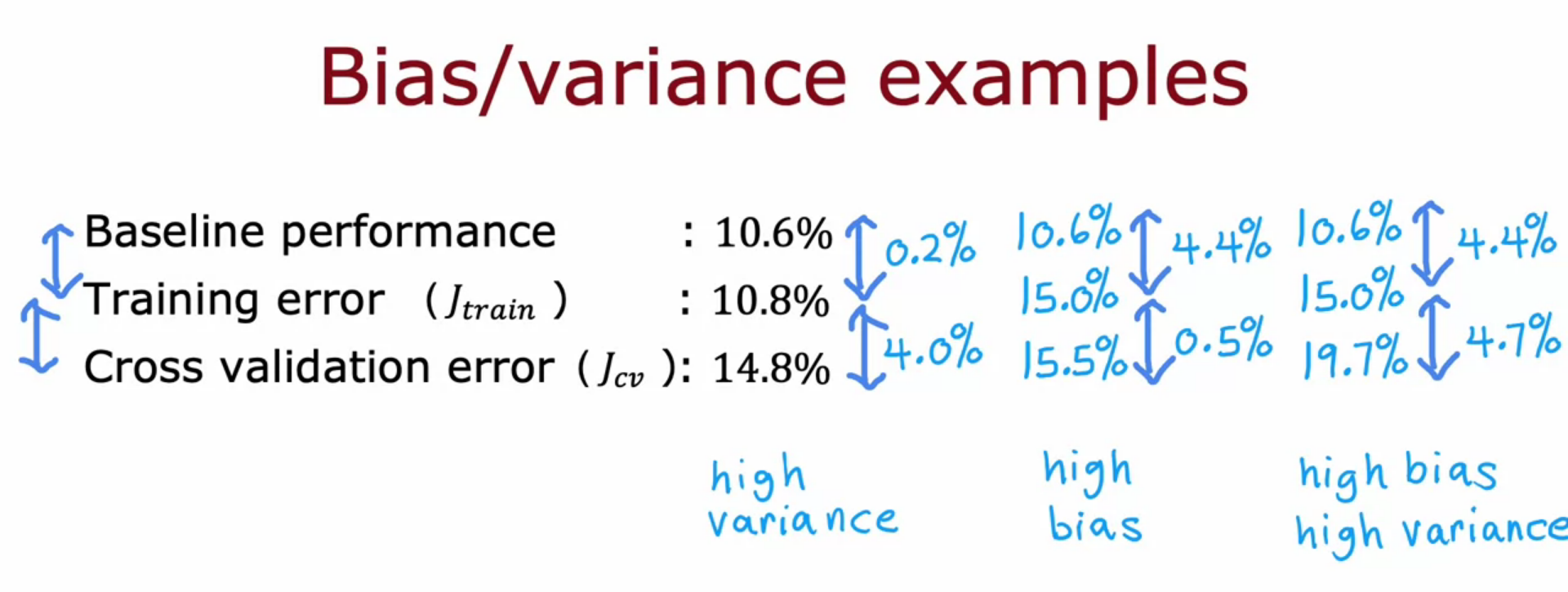
Baseline
- First find out the baseline performance human can achieve or default baseline
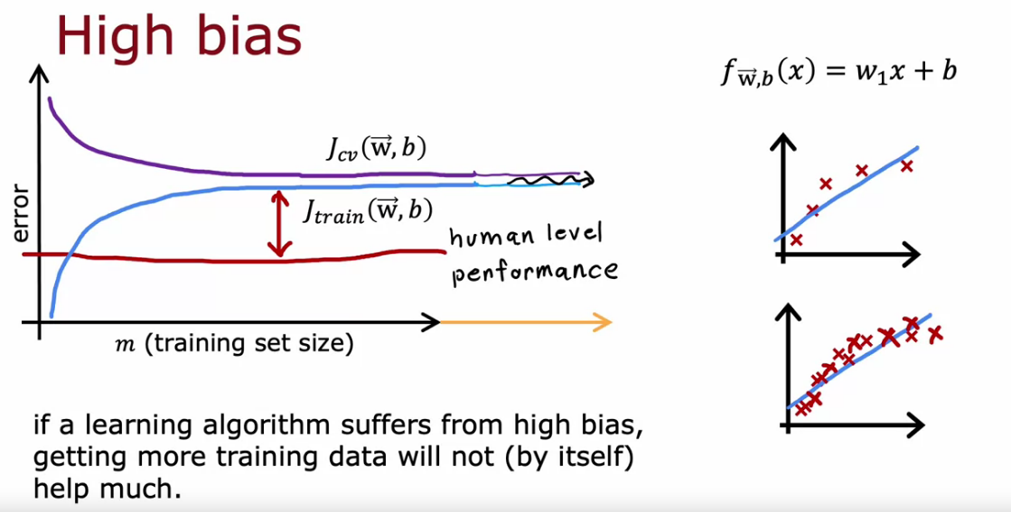
Learning Curve

If we have high bias increasing training data is not going to help. It wont decrease the error
If we have high variance increasing training data is going to help. It will decrease the error

Deciding what to try next revisited
BIAS
- Bias is the difference between the average prediction of our model and the correct value.
- Model with high bias pays very little attention to the training data and oversimplifies the model.
- It always leads to high error on training and test data.
VARIANCE
- Variance is the variability of model prediction for a given data point or a value which tells us spread of our data.
- Model with high variance pays a lot of attention to training data and does not generalize on test data.
- As a result, such models perform very well on training data but has high error rates on test data.
Overfitting - High Variance and Low Bias
Underfitting - High/Low Variance and High Bias
High Variance
- Get more training data - High Variance
- try increasing lambda - Overfit High Variance
- try small set of features - Overfit High Variance
High Bias
- try large set of features - Underfit High Bias
- try adding polynomial features - Underfit High Bias
- try decreasing lambda - Underfit High Bias
Bias and Variance Neural Networks
- Simple Model - High Bias
- Complex Model - High Variance
- We need a model between them, that is we need to find a trade off between them.
Neural Networks
- Large NN are having low bias machines
- GPU are there to speed up NN
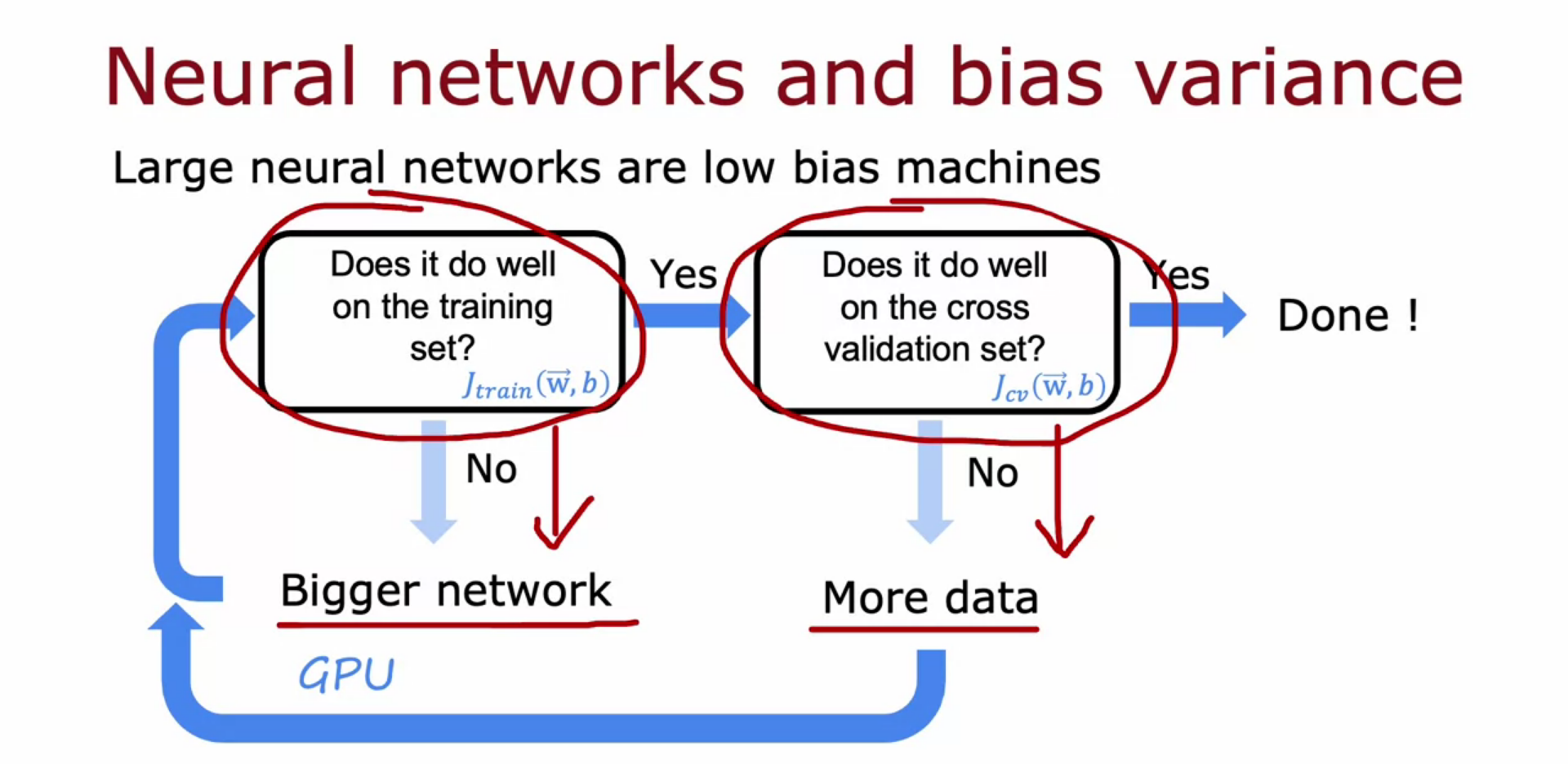

- With best Regularization large NN will do better than smaller one.
- But large NN take time to run
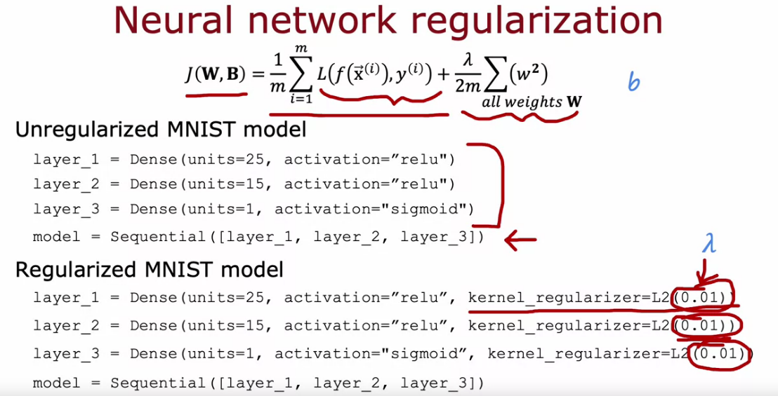
- Implementing NN with regularization having lambda 0.01 (L2 regularization Ridge)
Iterative loop of ML development
- Choose architecture - model and data
- train model
- diagnostic - bias, variance, error analysis

Error Analysis
- Manually (human) going through a misclassified small dataset and analyzing the data
- We get a idea about where to focus
Error analysis involves the iterative observation, isolating, and diagnosing erroneous Machine learning (ML) predictions.
In error analysis, ML engineers must then deal with the challenges of conducting thorough performance evaluation and testing for ML models to improve model ability and performance.
Error Analysis works by
- Identification - identify data with high error rates
- Diagnosis - enables debugging and exploring the datasets further for deeper analysis
- Model debugging
This deepcheck’s model error analysis check helps identify errors and diagnose their distribution across certain features and values so that you can resolve them.
from deepchecks.tabular.datasets.classification import adult
from deepchecks.tabular.checks import ModelErrorAnalysis

train_ds, test_ds = adult.load_data(data_format='Dataset', as_train_test=True)
model = adult.load_fitted_model()

# We create the check with a slightly lower r squared threshold to ensure that
# the check can run on the example dataset.

check = ModelErrorAnalysis(min_error_model_score=0.3)
result = check.run(train_ds, test_ds, model)
result

# If you want to only have a look at model performance at pre-defined
# segments, you can use the segment performance check.

from deepchecks.tabular.checks import SegmentPerformance
SegmentPerformance(feature_1='workclass',
									 feature_2='hours-per-week').run(validation_ds, model)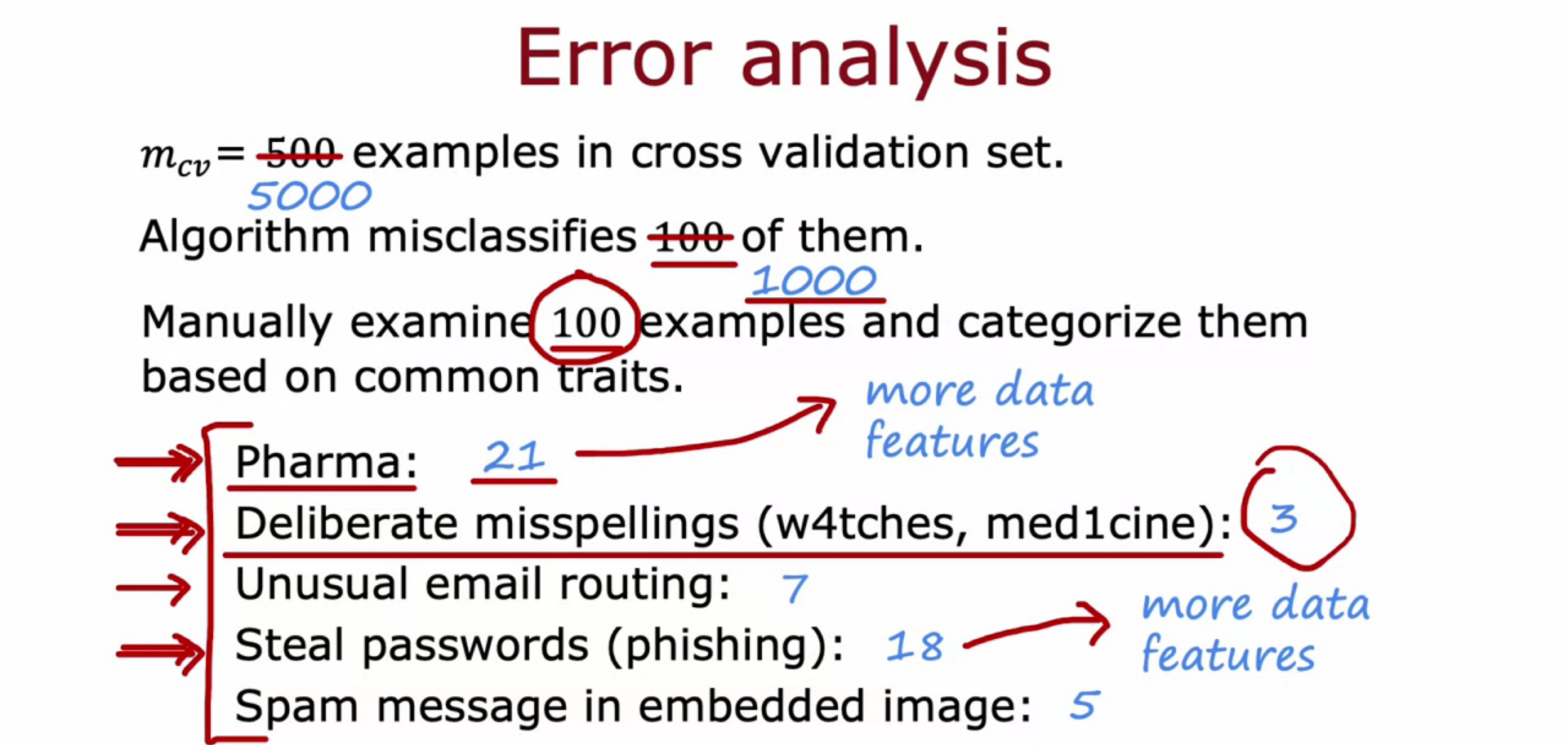
Adding Data
- Include data where error analysis pointed
Data Augmentation
Kind of feature engineering where we make more data from existing features
- Image Recognition
- rotated image
- enlarged image
- distorted image
- compressed image.
- Speech Recognition
- Original audio
- noisy background - crowd
- noisy background - car
- audio on a bad cellphone connection
For Image Text Recognition we can make our own data by taking screenshot of different font at different color grade
- Synthetic Data Creation is also now a inevitable part of majority projects.
- Focus on Data not the code
What is Transfer Learning ?
Transfer learning make use of the knowledge gained while solving one problem and applying it to a different but related problem (same type of input like, image model for image and audio model for audio.
For example, knowledge gained while learning to recognize cars can be used to some extent to recognize trucks.
- We want to recognize hand written digits from 0 to 9
- We change the last output layer we wanted from the large NN all ready pre build.
Pre Training
When we train the network on a large dataset(for example: ImageNet) , we train all the parameters of the neural network and therefore the model is learned. It may take hours on your GPU.
Fine Tuning
We can give the new dataset to fine tune the pre-trained CNN. Consider that the new dataset is almost similar to the orginal dataset used for pre-training. Since the new dataset is similar, the same weights can be used for extracting the features from the new dataset.
- If the new dataset is very small, it’s better to train only the final layers of the network to avoid overfitting, keeping all other layers fixed. So remove the final layers of the pre-trained network. Add new layers Retrain only the new layers.
- If the new dataset is very much large, retrain the whole network with initial weights from the pretrained model.
How to fine tune if the new dataset is very different from the orginal dataset ?
The earlier features of a ConvNet contain more generic features (e.g. edge detectors or color blob detectors), but later layers of the ConvNet becomes progressively more specific to the details of the classes contained in the original dataset.
The earlier layers can help to extract the features of the new data. So it will be good if you fix the earlier layers and retrain the rest of the layers, if you got only small amount of data.
If you have large amount of data, you can retrain the whole network with weights initialized from the pre-trained network.
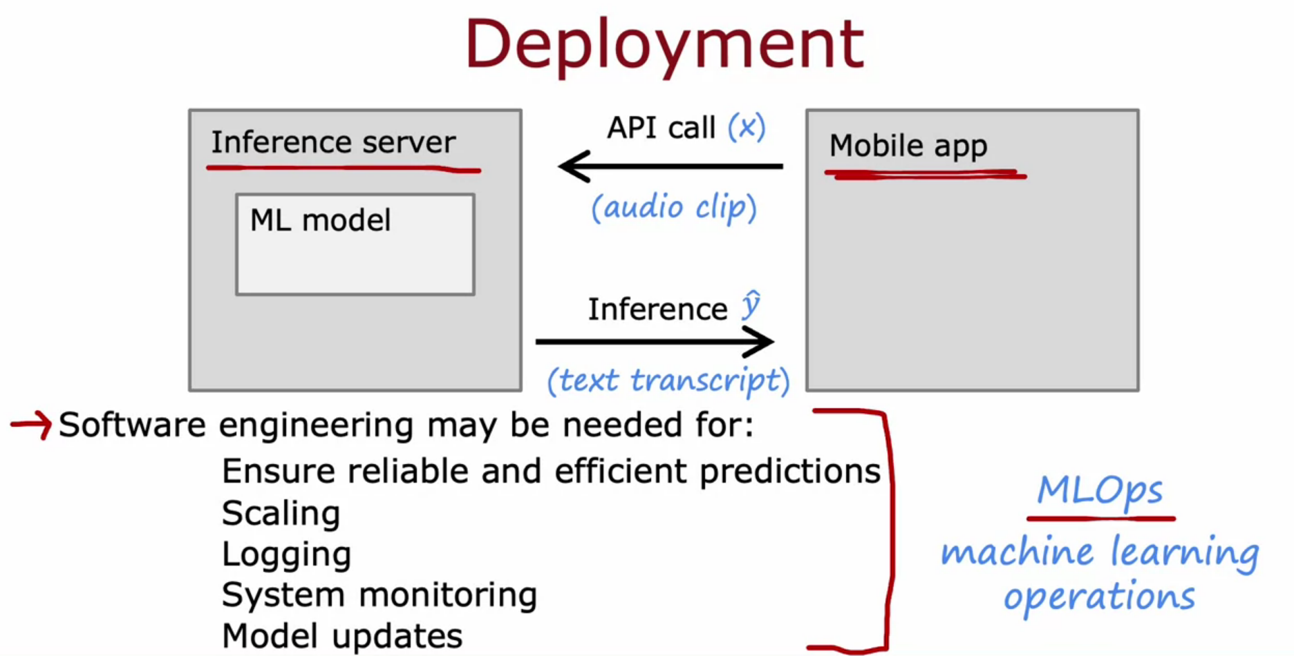
Full cycle of a machine learning project
- Define Project
- Define and Collect data
- Train/Error Analysis/Iterative Improvement
- Deploy Monitor and Maintain
Fairness, Bias, and Ethics
Bias
- Hiring tool to discriminate women.
- Facial Recognition system matching dark skinned individuals to criminal mugshot.
- Biased bank loan approval
- Toxic effect of reinforcing negative stereotypes
- Using DeepFakes to create national issues/political purpose
- Spreading toxic speech for user engagement
- Using ML to build harmful products, commit fraud etc
Guidelines
- Have a diverse team.
- Carry standard guidelines for your industry.
- Audit system against possible harm prior to deployment.
- Develop mitigation plan, monitor possible harm. (If self driving car get involved in accident)
Mitigation Plan - Reduces loss of life and property by minimizing the impact of disasters.
Error Metrics
- For classifying a rare disease, Accuracy is not best evaluation metrics
- Precision Recall and F1Score helps to measure the classification accuracy
Confusion Matrix in Machine Learning
Confusion Matrix helps us to display the performance of a model or how a model has made its prediction in Machine Learning.
Confusion Matrix helps us to visualize the point where our model gets confused in discriminating two classes. It can be understood well through a 2×2 matrix where the row represents the actual truth labels, and the column represents the predicted labels.
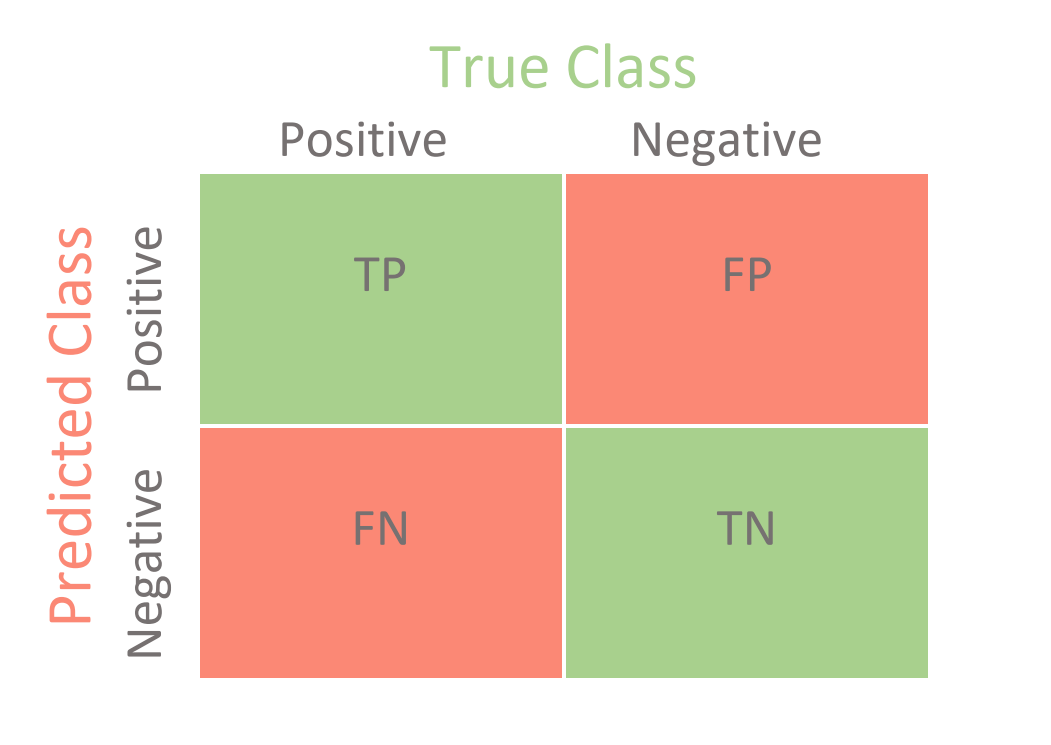
Accuracy
Simplest metrics of all, Accuracy. Accuracy is the ratio of the total number of correct predictions and the total number of predictions.
Accuracy = ( TP + TN ) / ( TP + TN + FP + FN )
Precision
Precision is the ratio between the True Positives and all the Positives. For our problem statement, that would be the measure of patients that we correctly identify having a heart/rare disease out of all the patients actually having it.
Eg : Suppose I predicted 10 people in a class have heart disease. Out of those how many actually I predicted right.
Precision = TP / ( TP + FP )
Recall
The recall is the measure of our model correctly identifying True Positives. Thus, for all the patients who actually have heart disease, recall tells us how many we correctly identified as having a heart disease.
Eg : Out of all people in a class having heart disease how many I got right prediction.
Recall = TP / ( TP + FN )
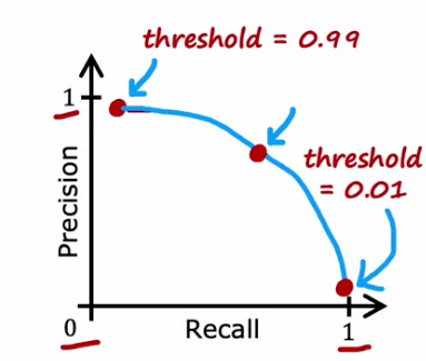
Trading off Precision and Recall
- If we want to predict 1 (rare disease) only if we are really confident, then
- High Precision and Low Recall
- We set high threshold, predict 1 if f(x) ≥ 0.99
- If we want to predict 1 (rare disease) when in small doubt, then
- Low Precision and High Recall
- We set small threshold, predict 1 if f(x) ≥ 0.01
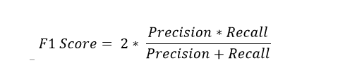
F1 Score
For some other models, like classifying whether a bank customer is a loan defaulter or not, it is desirable to have a high precision since the bank wouldn’t want to lose customers who were denied a loan based on the model’s prediction that they would be defaulters.
There are also a lot of situations where both precision and recall are equally important. For example, for our model, if the doctor informs us that the patients who were incorrectly classified as suffering from heart disease are equally important since they could be indicative of some other ailment, then we would aim for not only a high recall but a high precision as well.
In such cases, we use something called F1-score is used . F1-score is the Harmonic mean of the Precision and Recall
Precision, Recall and F1 Score should be close to one, if it is close to zero then model is not working well. (General case)
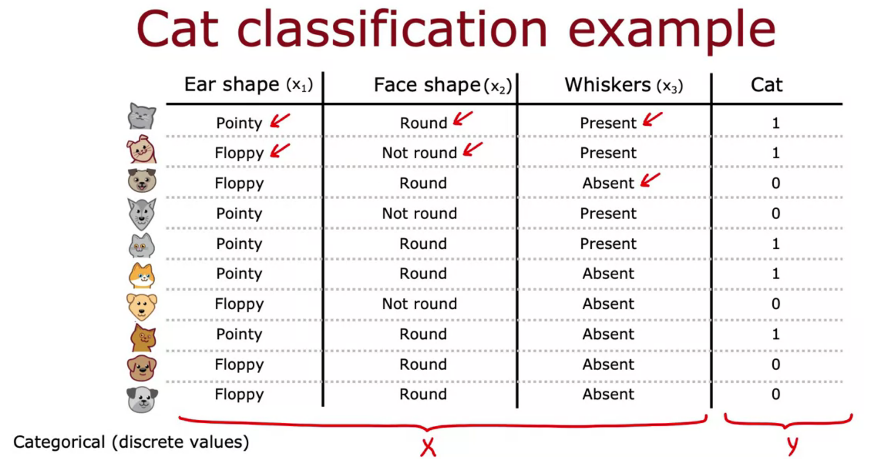
Decision Tree Model
- If features are categorical along with a target, for a classification problem decision tree is a good model
- Starting of DT is called Root Node
- Nodes at bottom is Leaf Node
- Nodes in between them is Decision Node
- The purpose of DT is to find best tree from the possible set of tree


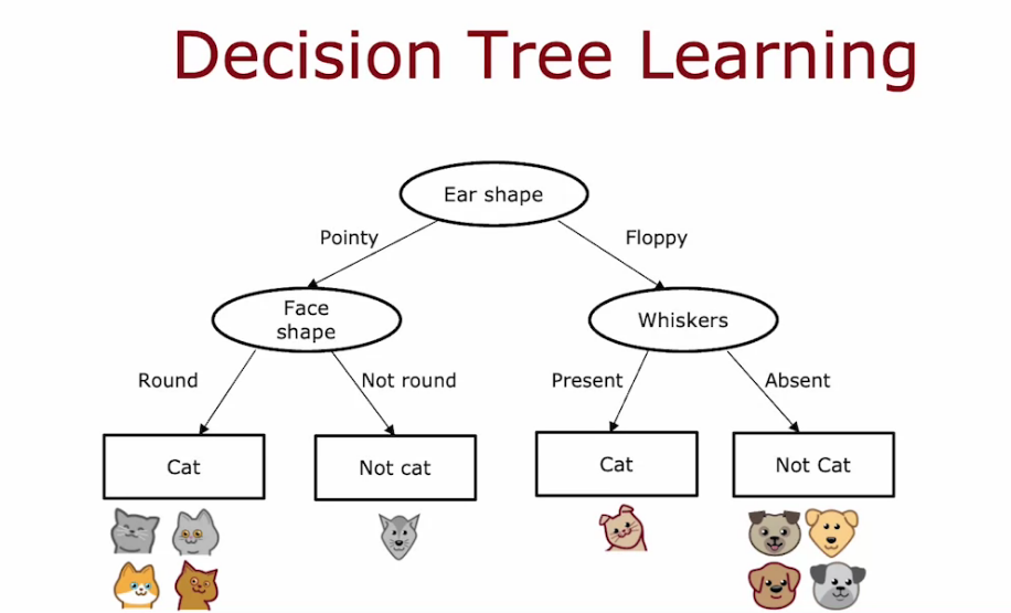
Decision Tree Learning Process
- If we reach at a node full of specific class, we stop there and set the node as leaf node.
- we want to achieve purity, that is class full of same type (Not completely possible all time).
- In order to maximize the purity, we need to decide where we need to split on at each node.
When to stop splitting?
- When node is 100% one class
- Reaching maximum depth of tree
- When depth increases - Overfitting
- When depth decreases - Underfitting
- when impurity score improvements are below a threshold
- Number of examples in a node is below a threshold
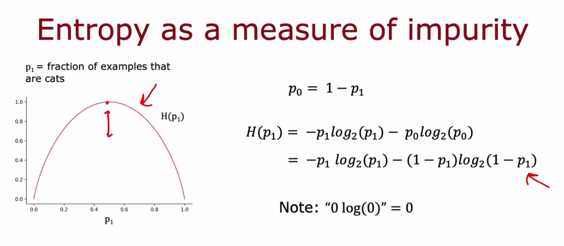
Measuring Purity
- Entropy is measure of Impurity/randomness in data
- It starts from 0 to 1 then goes back to 0
- P1 is the fraction of positive examples that are same class
- P0 is opposite class
- Entropy equation is as follows;
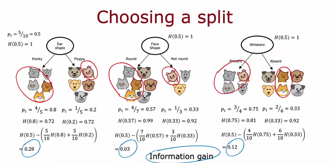
Choosing a split: Information Gain
Reduction of Entropy is Information Gain
Some Initial Steps
- We calculate the Entropy in each decision node - Low Entropy is Good, Shows Less Impurity
- Also number of elements in sub branch is also important - High Entropy in Lot of Samples is Worse
- We need to combine the Entropy of two side somehow
- First calculate product of ratio of elements in node with Entropy. Take sum of both of that value from each side.
- Subtract from root node P1
By this we get reduction in entropy know as Information Gain. Then pick the largest Information gain for best output in decision tree.

Putting it together
- Start with all examples at root node
- Calculate Information Gain for all features and pick one with large IG
- Split data into left and right branch
- keep repeating until,
- Node is 100% one class
- When splitting result in tree exceeding depth. Because it result in Overfitting
- If information gain is less than a threshold
- if number of examples in a node is less than a threshold
Decision Tree uses Recursive Algorithm
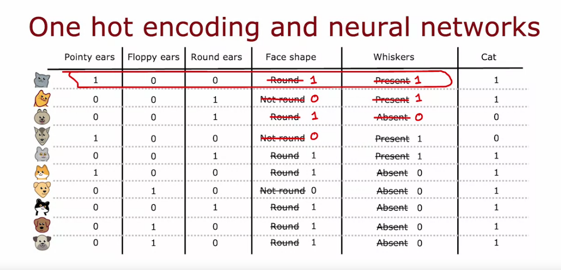
Using one-hot encoding of categorical features
- One hot encoding is a process of converting categorical data variables to features with values 1 or 0.
- One hot encoding is a crucial part of feature engineering for machine learning.
- In case of binary class feature we can covert in just one column with either 0 or 1
- Can be used in Logistic/Linear Regression or NN
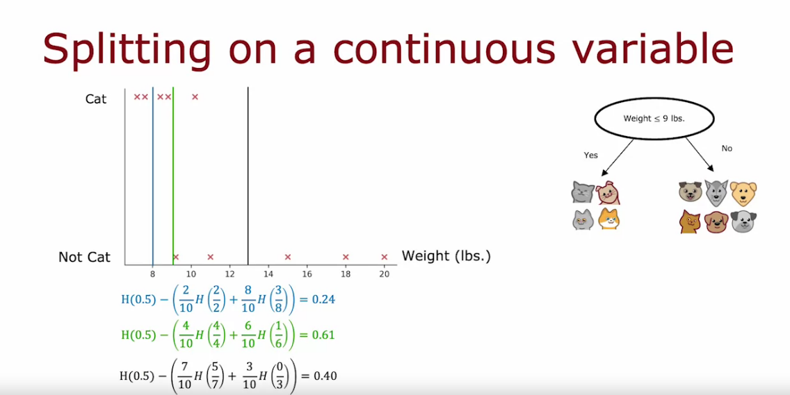
Decision Tree for Continuous valued features
- Below example weight is continuous
- We can consider weight ≤ x lbs, to split into 2 classes
- The value of x can be changed and calculate Information Gain for each case.
- General case is to use 3 cases but can be changed.
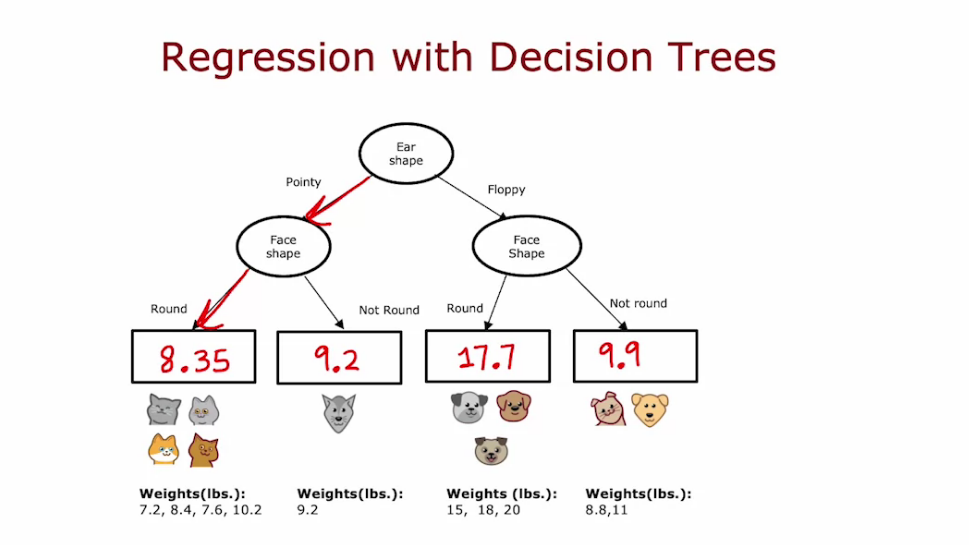
Regression Trees
- It is same as Decision problem. At the end when we reach leaf node we calculate the average and predict
- But instead of Information Gain we calculate Reduction in Variance
- Calculate the variance of the leaf node then multiply by the ratio of number of elements, finally subtract it from variance of root node
- We choose split which give Largest Reduction in Variance

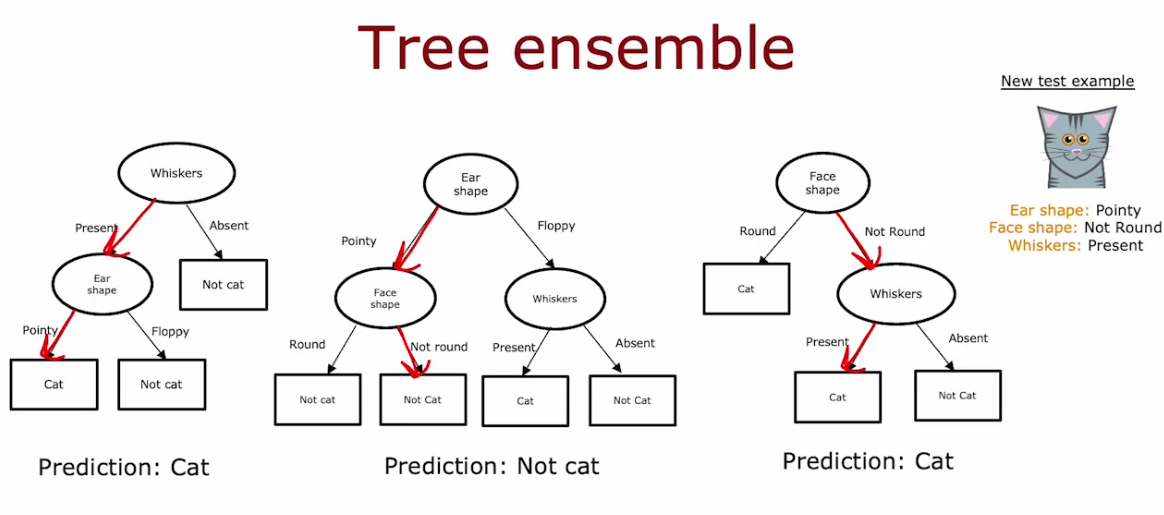
Using Multiple Decision Trees
- To avoid the sensitivity and make model robust we can use Multiple Decision Tree called Tree ensembles (collection of multiple tree)
- We take majority of the Ensemble prediction
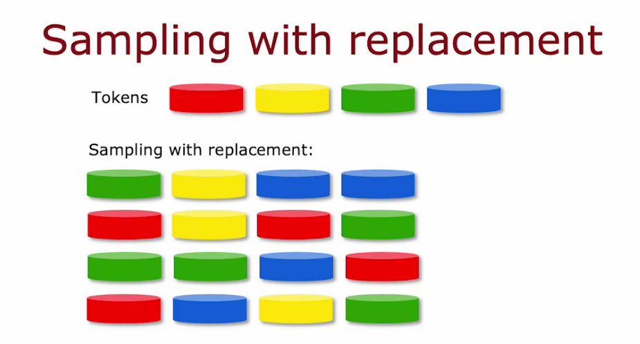
Sampling with replacement
- Help to construct new different but similar training set.

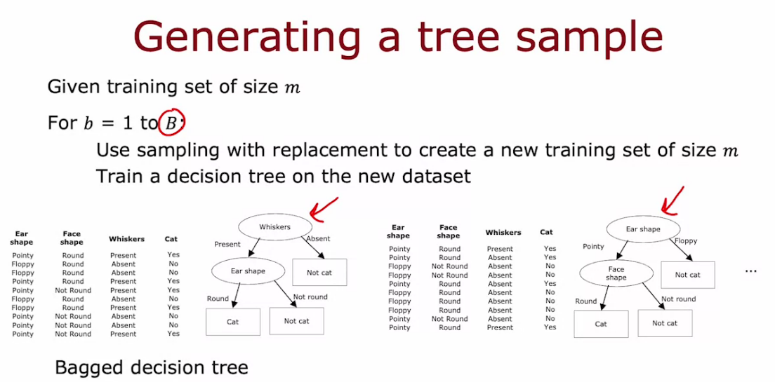
Random Forest Algorithm
- Pick a train data
- make duplicate of train data using sampling by replacement technique, Increasing this number of synthetic samples is ok. It do improve performance. But after a limit it is just a waste of GPU.
- Since we create new Decision Tree using this technique, it is also called Bagged Decision Tree
- Sampling helps Random Forest to understand small changes.
- Using different Decision Tree and averaging it improve robustness of Random Forest
Suppose that in our example we had three features available rather than picking from all end features, we will instead pick a random subset of K less than N features. And allow the algorithm to choose only from that subset of K features. So in other words, you would pick K features as the allowed features and then out of those K features choose the one with the highest information gain as the choice of feature to use the split. When N is large, say n is Dozens or 10's or even hundreds. A typical choice for the value of K would be to choose it to be square root of N.
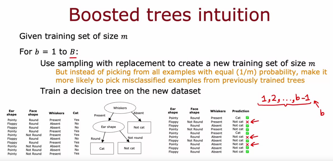
XGBoost
- Same like Random Forest, but in sampling while choosing next sample, we give more preference for picking the wrongly predicted one in the First made Decision Tree.

# Classification
from xgboost import XGBClassifier
model = XGBClassifier()
model.fit(x_train, y_train)
y_pred = model.predict(x_test)

# Regression
from xgboost import XGBRegressor
model = XGBRegressor()
model.fit(x_train, y_train)
y_pred = model.predict(x_test)
When to use Decision Trees
| Decision Tree and Tree Ensembles | Neural Networks |
|---|---|
| Works well on tabular data | Works well on Tabular ( Structured and Unstructured data) |
| Not recommended for Images, audio and text | Recommended for Image, audio, and text |
| fast | slower than DT |
| Small Decision tree may be human interpretable | works with transfer learning |
| We can train one decision tree at a time. | when building a system of multiple models working together, multiple NN can be stringed together easily. We can train them all together using gradient descent. |
Unsupervised Learning, Recommenders, Reinforcement Learning - Course 3
What is Clustering?
- Clustering is used to group unlabeled data
- There are various algorithms to perform the Clustering.
K- Means Intuition
- K is the decided number of clusters by us.
- Pick 2 random point
- These 2 point form center of cluster called Cluster Centroids
- After classifying like that it finds the average/mean
- Move all Cluster Centroids to that average/mean point
- Repeat the process for that Cluster Centroids
- After repeating it for a time period we finally get a Cluster Centroids where further repeating don’t make any change.
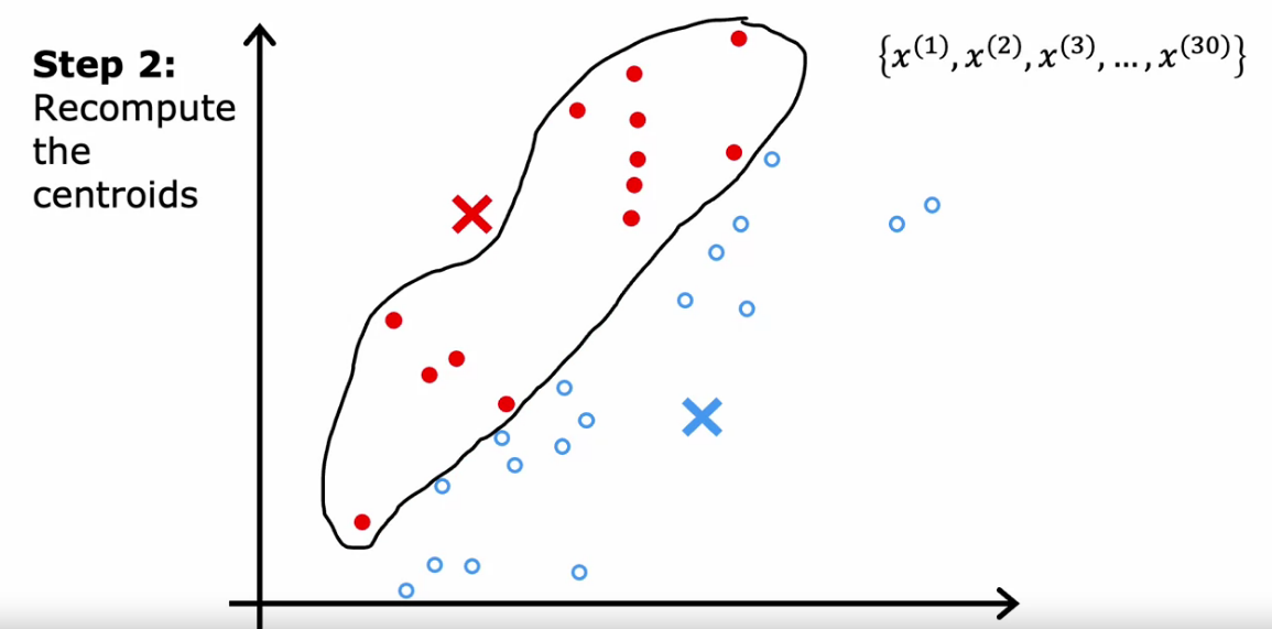


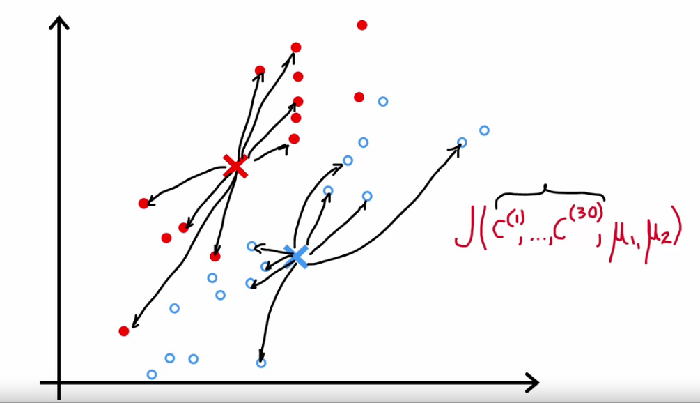
K-means Algorithm
- Find minimum value of Norm of each points with the Clustering Centroid
- Then find and mark the clusters
- Find average of cluster and move Clustering Centroid to that mean
- Repeat process
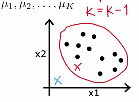
- If no sample assigned to a cluster. We can’t move forward. Because we will be trying to find average of zero points.
- So we can eliminate that cluster, Or Reinitialize that K-means
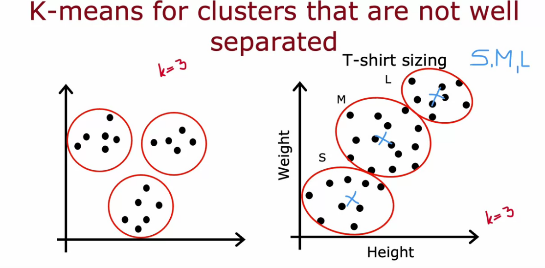
K - Means can be also helpful for data that are not that much separated
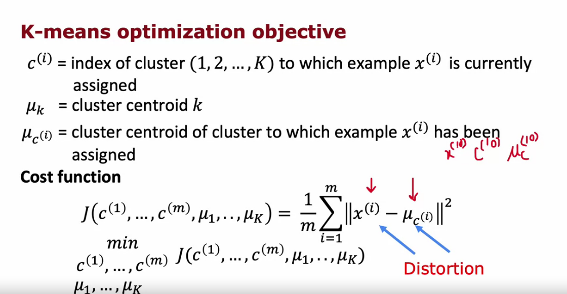
Optimization objective of K-Means - Distortion Function
- Here also we try to minimize the a Cost Function called Distortion Function
- We calculate average of squared, difference of distance
- we want to minimize the cost function
Since we are moving cluster centroid to mean and calculating cost function really shows a decrease than previous one. So it is sure that distortion function, cost function goes down and goes to convergence. So no need to run the K-means if distortion change is less than a small threshold. It means it reached convergence.

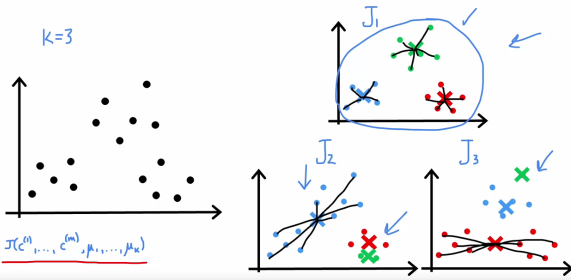
Initializing K-means
- First we need to pic a random points as cluster centroids
- Choose number of Cluster Centroid < Number of sample, K < m
- So pick K examples from the data
- Different Initialization give different result, we need to pic the one with Min Cost Function (Distortion)

Choosing the Number of Clusters
- Number of Clusters really ambiguous
- Our ultimate aim is not to pick really small Cost Function. In that case we can directly use large K to solve issue
- We really want to pick K that really make sense
- We can decide manually what k to pick based on Image Compression we want.
Types of method to choose value of K
Elbow Method
- We plot the Cost Function for different K
- It will look like Elbow
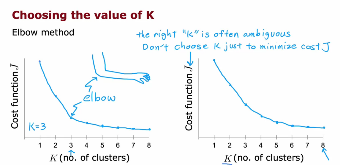

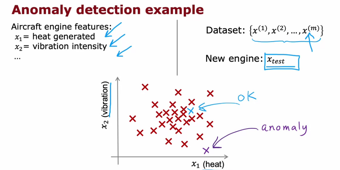
Anomaly Detection
- It is basically finding unusual things in data.
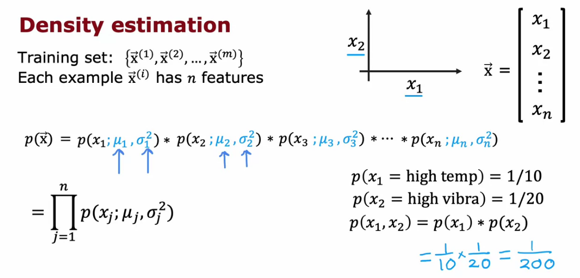
- We can perform Anomaly Detection using Density Estimation
- We can find the probability of the testing data and if it is less than the threshold epsilon, It is unusual, If it is greater than the epsilon it is normal

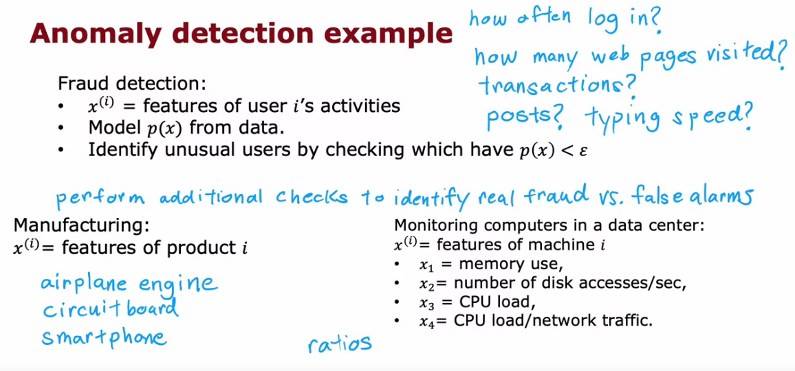
Fraud Detection and in Manufacturing Checking
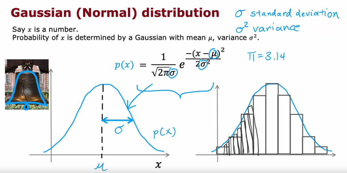
Gaussian (Normal) Distribution
- It is also called bell shaped curve
- When width of sigma (standard deviation) increases then the values is spread out
- When width of sigma decreases then the values are close together


Anomaly Detection Algorithm


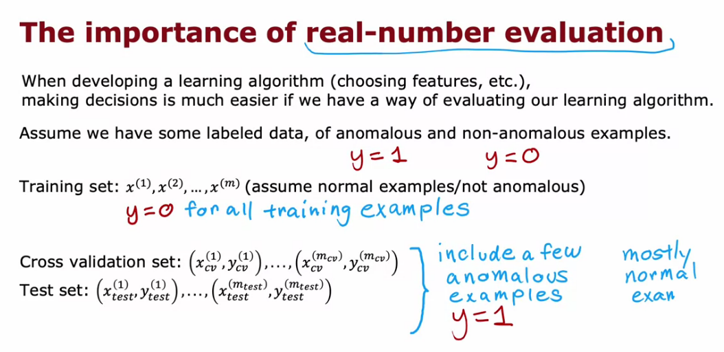
Developing and evaluating an anomaly detection system
- Even if we a labelled data by assumption, anomaly can be applied to find the real anomaly out of wrongly labelled data


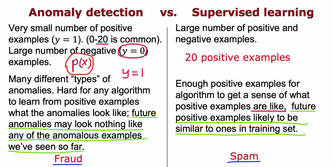
Anomaly detection vs. supervised learning
Anomaly is flexible than SL, because in SL we are learning from the data that is available. If something happened out of the box, SL cannot catch that but Anomaly can.

Choosing What Features to Use
- Anomaly like features with Gaussian Distribution
- To make features gaussian we can make use of log and other polynomial transformation.
# Feature transformations to make it gaussian
plt.hist(np.log(x+1), bins=50)
plt.hist(x**0.5, bins=50)
plt.hist(x**0.25, bins=50)
plt.hist(x**2, bins=50)

# In code bins is changed to make histogram less box type.
# Width of histograms decreases as bins increases.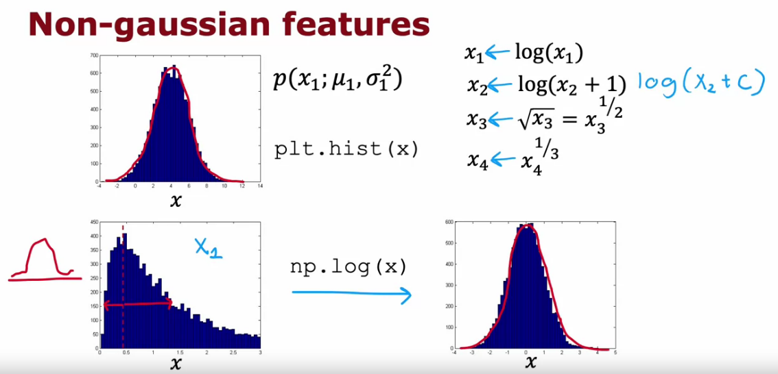


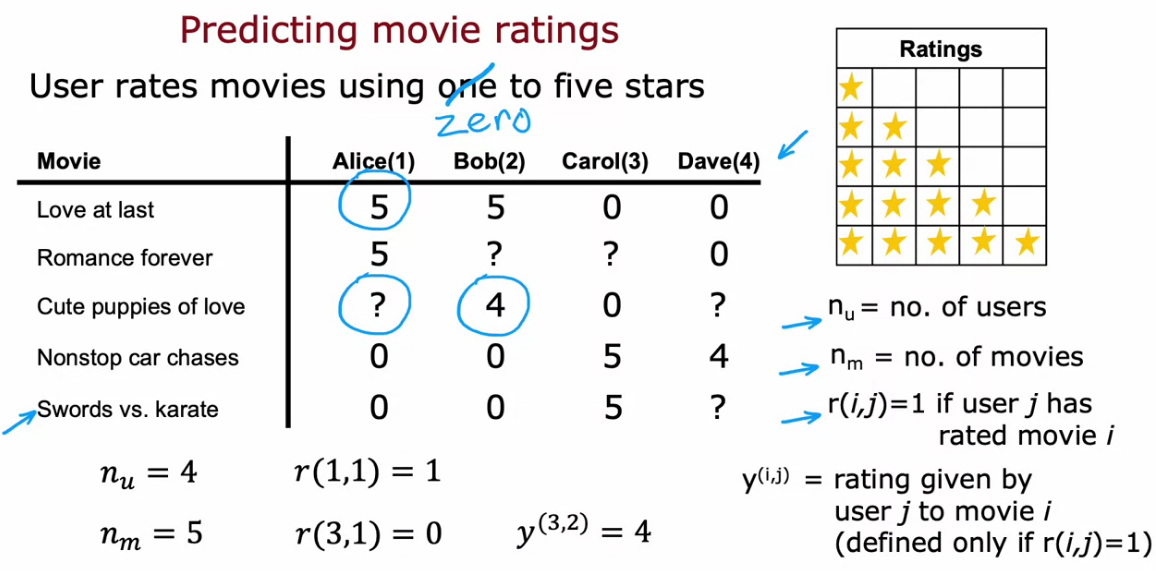
Making Recommendations
- Amazon/Netflix every company now uses recommender systems
- Here we try to find the movies they have not rated, then we predict the rating for that movie and recommend it to the user if the predicted rating is 5 star.
Using per-item features
- It is more like Linear Regression. But here we usually add Regularization along with that.
- Here also we calculate the cost function and try to minimize the Cost Function
- Suppose that we have features of movies, for that vector we need to find the w and be for a user to predict ratings of any movies
- So we need to find the parameters w and b
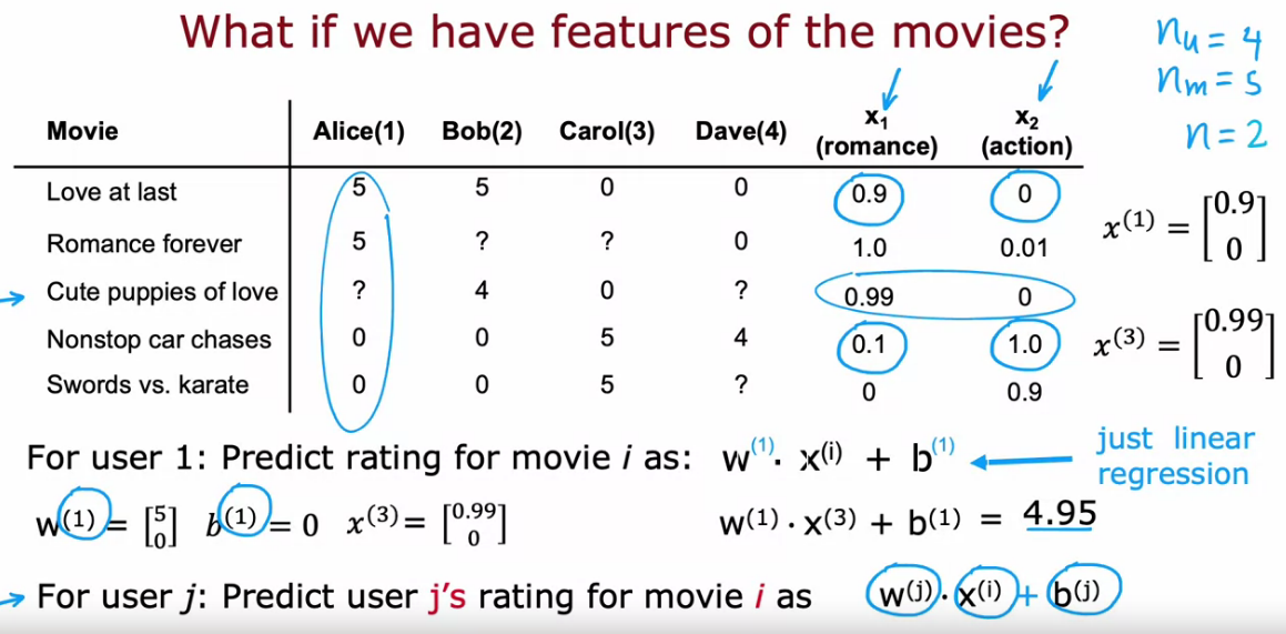
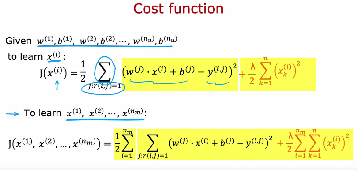
- To find the W and b, we find and try to minimize the cost function
- For cost function we use MSE plus the L2 regularization
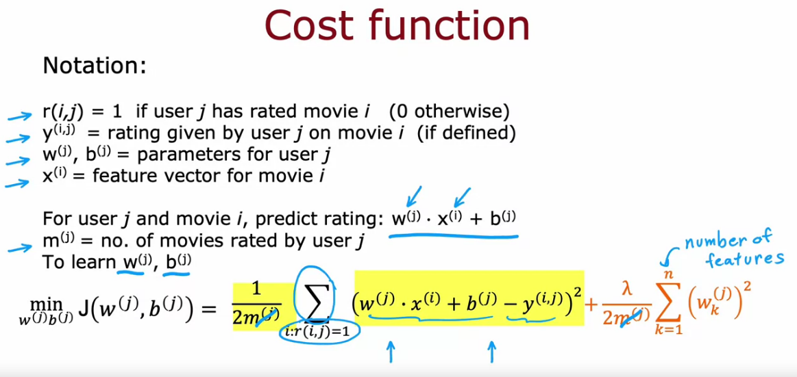
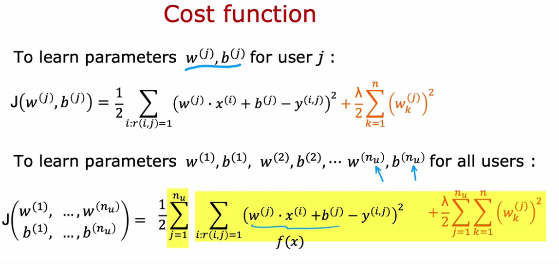
- But we need to learn the parameters for all users
- So the cost function need a little modification.
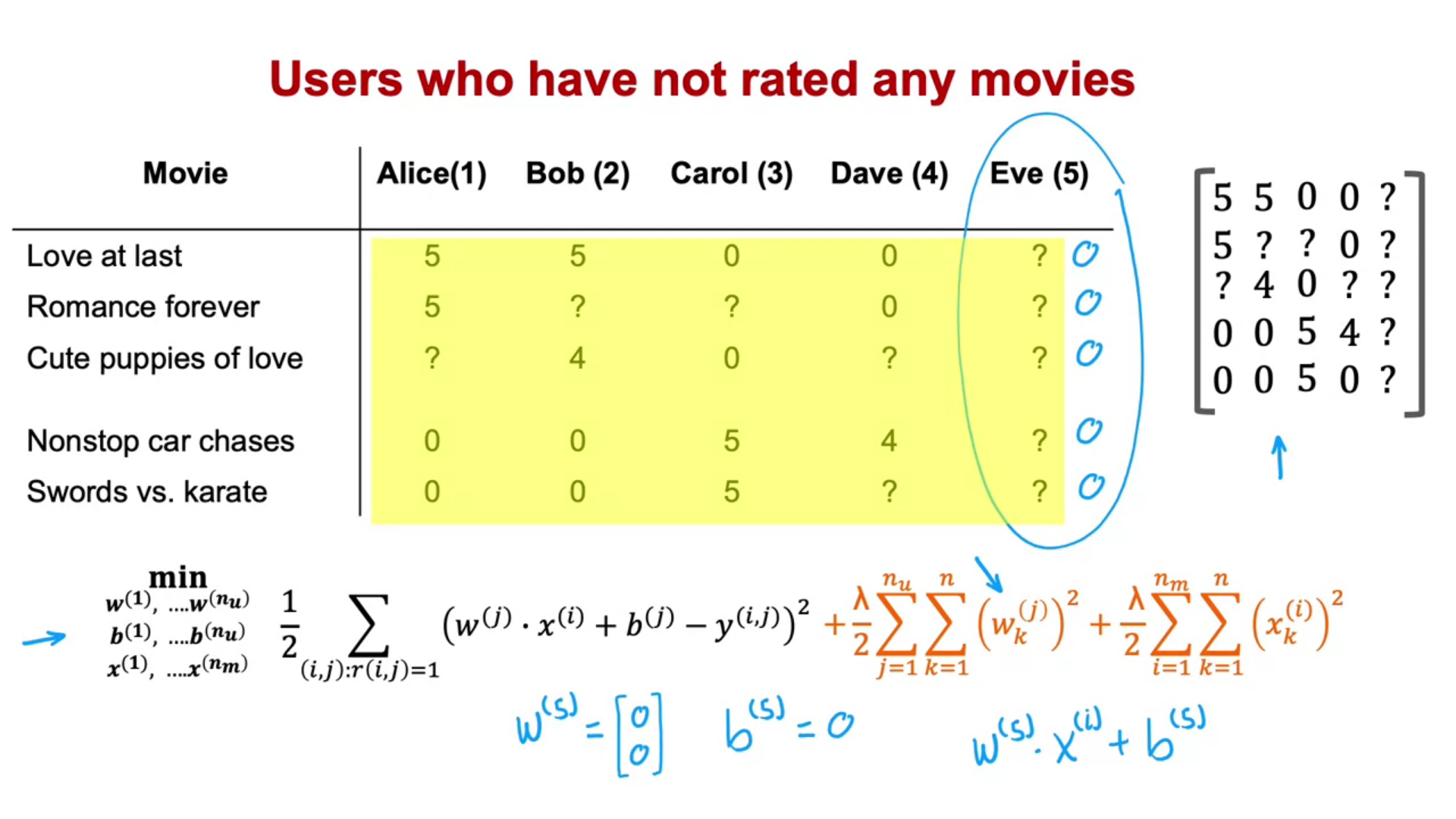
- What to do if we don’t have the features data
- Suppose we already learned the parameters W and b, then comparing with the ratings of movie by users we can find the features.
- Now by using that features we can predict the ratings of un rated movies by users
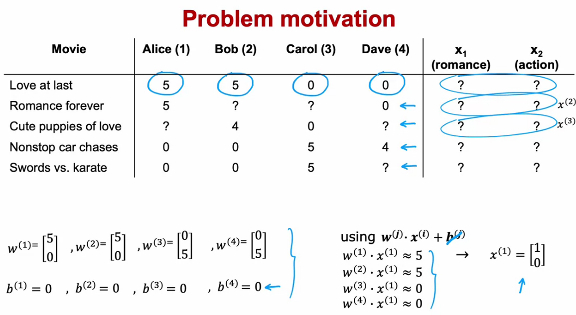
- To learn the features, the cost function is given below
- In order to generalize the cost function, we try to learn for all users
Collaborative filtering algorithm
Collaborative filtering refers to the sense that because multiple users have rated the same movie collaboratively, given you a sense of what this movie maybe like, that allows you to guess what are appropriate features for that movie, and this in turn allows you to predict how other users that haven't yet rated that same movie may decide to rate it in the future.
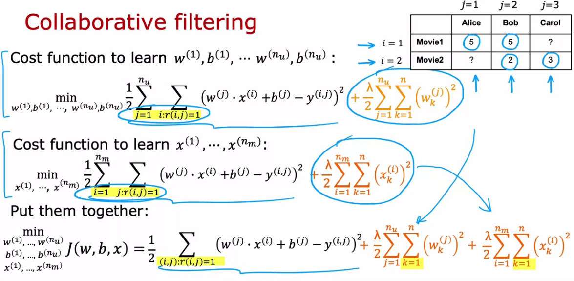
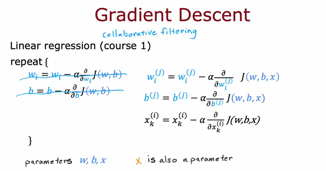
- Now the cost function is a function of W, b and x
- So while applying gradient descent we need to use it in x also.
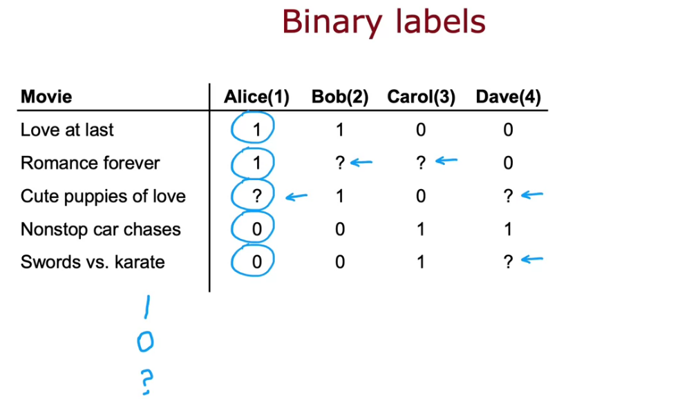
Binary labels: favs, likes and clicks
So far, our problem formulation has used movie ratings from 1- 5 stars or from 0- 5 stars. A very common use case of recommended systems is when you have binary labels such as that the user favors, or like, or interact with an item. A generalization of the model that you've seen so far to binary labels.
- So we can convert linear regression to logistic regression model. So MSE cost function changes to Log Loss


Mean Normalization
- Subtract the mean (average rating) from the rows, which is each user rating.
- So the movies not rated by user is replaced by average rating. This is Normalization.

TensorFlow Implementation of Collaborative Filtering
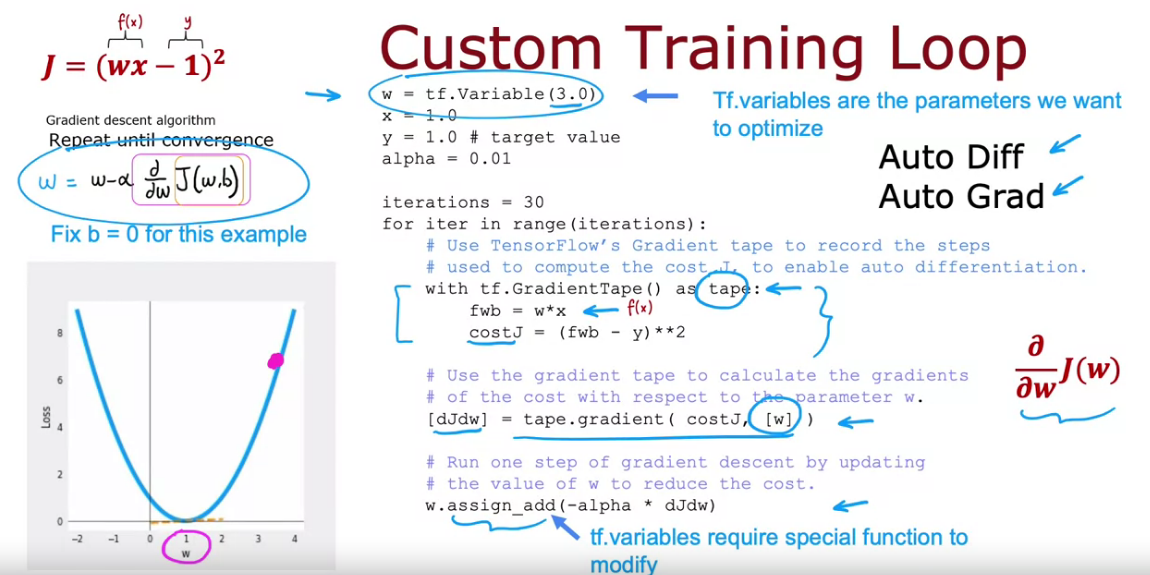
# Instantiate an optimizer.
optimizer = keras.optimizers.Adam (learning_rate=le-1)
iterations = 200
for iter in range (iterations):
# Use TensorFlow's GradientTape
# to record the operations used to compute the cost
with tf. GradientTape () as tape:
# Compute the cost (forward pass is included in cost)
cost value = cofiCostFuncV (X, W, b, Ynorm, R, num_users, num movies, lambda)
# Use the gradient tape to automatically retrieve
# the gradients of the trainable variables with respect to the loss
grads = tape.gradient( cost_value, [X,W,b] )
# Run one step of gradient descent by updating
# the value of the variables to minimize the loss.
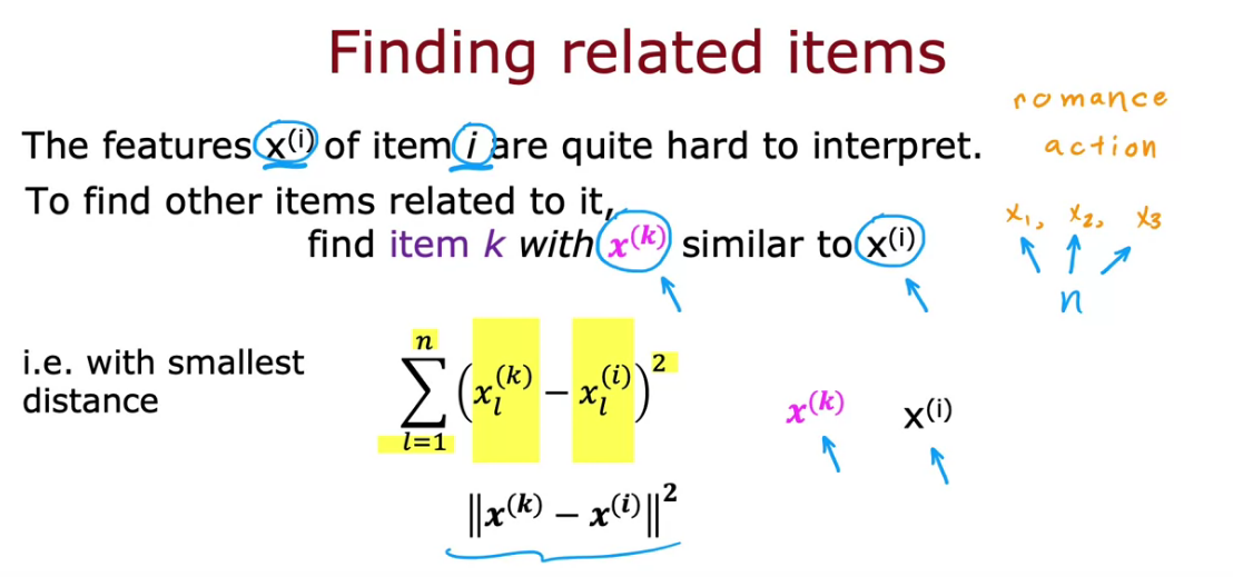
optimizer.apply_gradients( zip (grads, [X,W,b]) )Finding Related Items
- In all cases for recommending something, we need to find the relation between the items.
- Collaborative Filtering can find relation, using MSE between items. But has so many limitation.
Limitations of Collaborative Filtering
- Cold start problem How to
- rank new items that few users have rated?
- Use side information about items or users:
- Item: Genre, movie stars, studio,
- User: Demographics (age, gender, location), expressed preferences….
Collaborative filtering vs Content-based filtering
- Collaborative - Recommend items to you based on ratings of users who gave similar ratings as you.
- Content-based - Recommend items based on features of user and item to find good match.
Examples of user and item features
The features User and Movie can be clubbed together to form a vector.
User Features
- Age
- Gender
- Country
- Movie Watched
- Average rating per genre
Movie Feature
- Year
- Genre/Genres
- Reviews
- Average Rating
To predict the movie rating we can use a linear regression were w can be heavily depend on user feature vector and x can depend on movie feature vector.
For this we need vectors for User and Movies
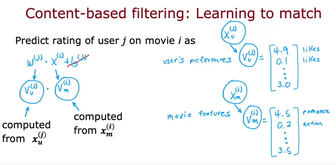
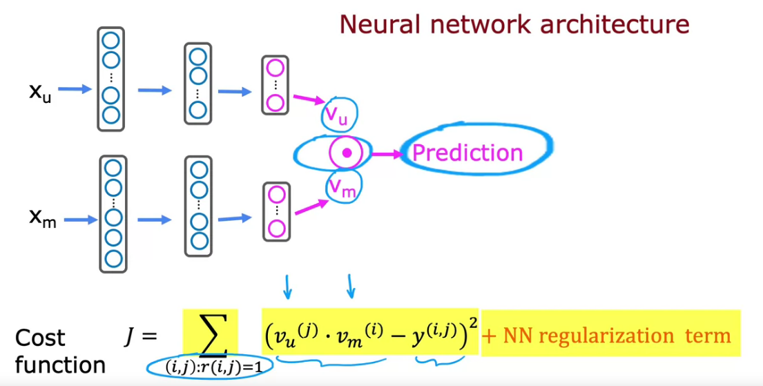
Deep learning for content-based filtering
- For User and Movie features we need to create vectors
- First NN will be User Network, Output Vu, which is a Vector of User
- Second NN will be Movie Network, Output Vm, which is a Vector of Movie
- Both output Vu and Vm have same dimension. Using that we create the cost function
- Since various NN can be linked together easily, we can take product of both user and movie vector.

Recommending from a large catalogue
We always have large set of items when it comes to Movies. Songs, Ads, Products. So having to run NN instance for millions of times whenever user log in to system is difficult.
So there are two steps
Retrieval
- Generate large list of plausible (probable) item of candidate
- For last 10 movies watched by user, find 10 most similar movies
- For most viewed genre find top 10 movies
- Top 20 movies in the country
- Combined Retrieved items to list, removing duplicates, items already watched, purchased etc
Ranking
- Take list retrieved and rank them based on learned model
- Display ranked items to user
Retrieving more items results in better performance, but slower recommendations
To analyze that run it offline and check if recommendation, that is p(y) is higher for increased retrieval.
Ethical use of recommender systems
What is the goal of the recommender system?
- Movies most likely to be rated 5 stars by user
- Products most likely to be purchased
Illegal Things
- Ads most likely to be clicked on
- Products generating the largest profit
- Video leading to maximum watch time
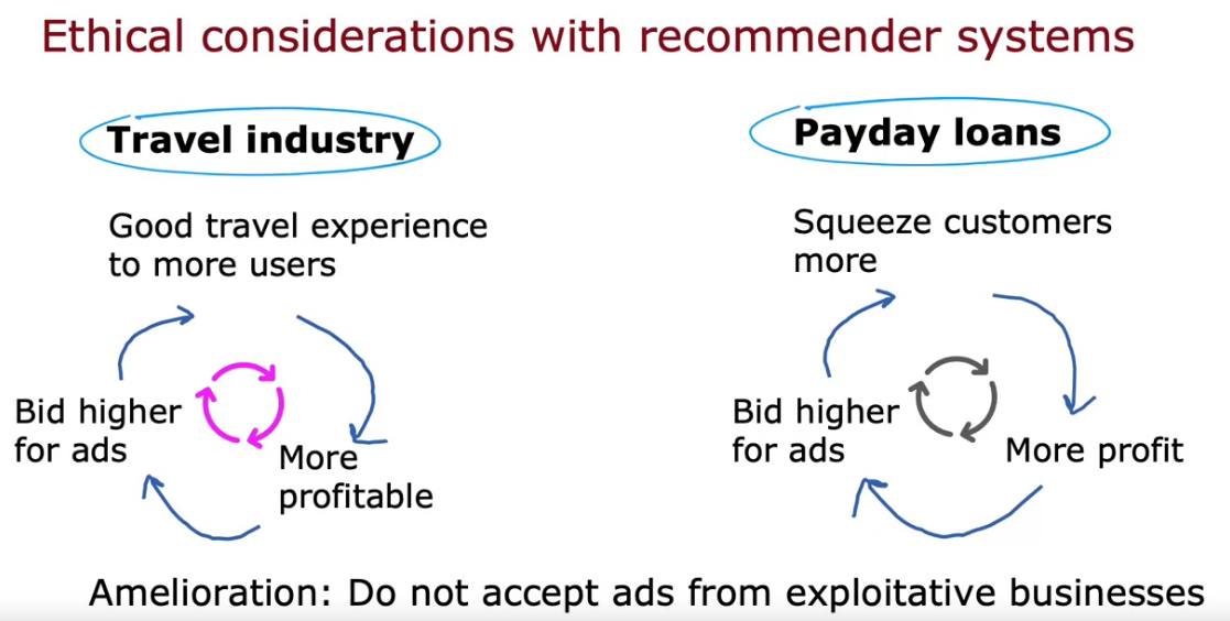
Other problematic cases:
- Maximizing user engagement (e.g. watch time) has led to large social media/video sharing sites to amplify conspiracy theories and hate/toxicity
- Amelioration: Filter out problematic content such as hate speech, fraud, scams and violent content
- Can a ranking system maximize your profit rather than users' welfare be presented in a transparent way
- Amelioration: Be transparent with users
TensorFlow implementation of content-based filtering
First create the 2 NN of user and movie/item
user_NN = tf.keras.models. Sequential ([
													 tf.keras.layers.Dense (256, activation='relu'),
													 tf.keras.layers.Dense (128, activation=' relu'),
													 tf.keras.layers.Dense (32)
												])
item NN = tf.keras.models. Sequential ([
													 tf.keras.layers.Dense (256, activation= 'relu'),
													 tf.keras.layers.Dense (128, activation= 'relu'),
													 tf.keras.layers.Dense (32)
])- Now we need to combine both Vm and Vu
- So we take user_NN and item_NN as input layer of combined model
- Then take their product to make output
- Prepare the model using this NN
- Finally evaluate model by MSE cost function to train the model
# create the user input and point to the base network
input_user = tf.keras.layers. Input (shape=(num_user_features))
vu = user_NN (input_user)
vu = tf.linalg.12_normalize (vu, axis=1)
# create the item input and point to the base network
input_item = tf.keras.layers. Input (shape=(num_item_features))
vm = item_NN (input_item)
vm = tf.linalg.12_normalize (vm, axis=1)
# measure the similarity of the two vector outputs
output = tf.keras.layers. Dot (axes=1) ([vu, vm])
# specify the inputs and output of the model
model = Model ([input_user, input_item], output)
# Specify the cost function
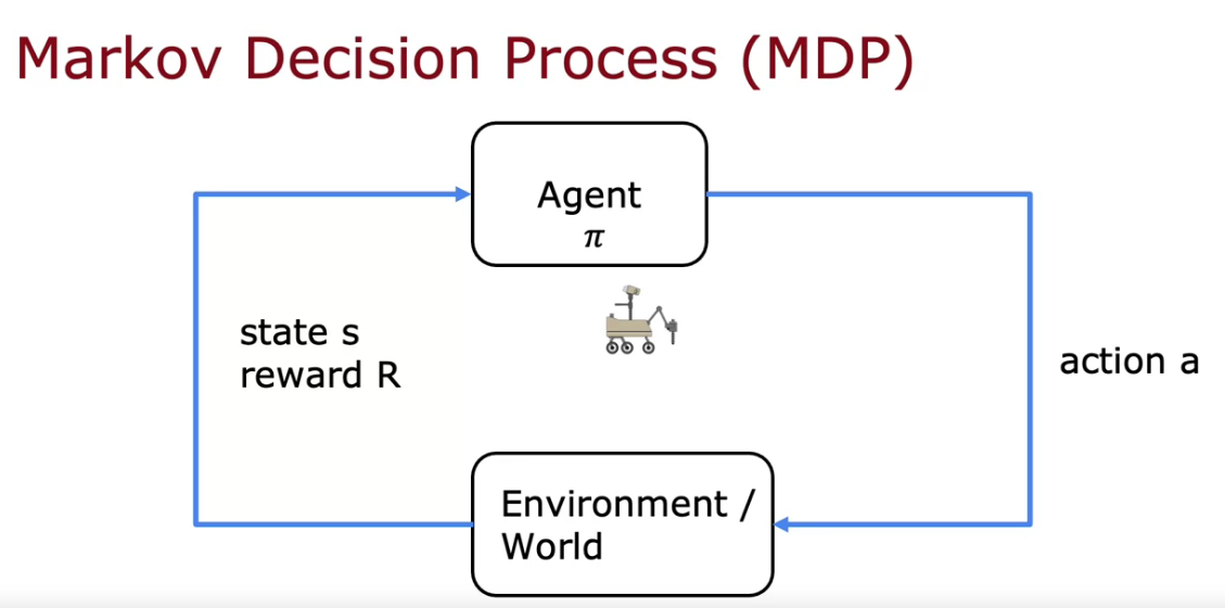
cost_fn= tf.keras.losses. Mean SquaredError ()What is Reinforcement Learning?
- Here we try to perform a action from it’s given state
- We can use the linear relation too, but it is not possible to get the dataset of the input x and output y
- So supervised learning won’t work here.
- Here we tell the model what to do. But not how to do
- We can make the mark the data as 1 if it performs well and -1 if it fails
- Algorithm automatically figure out what to do. We just need to say to the algorithm, if it is doing well or not using data input.
Applications
- To Fly a Helicopter
- Control Robots
- Factory Optimization
- Stock Trading
- Play Video Games
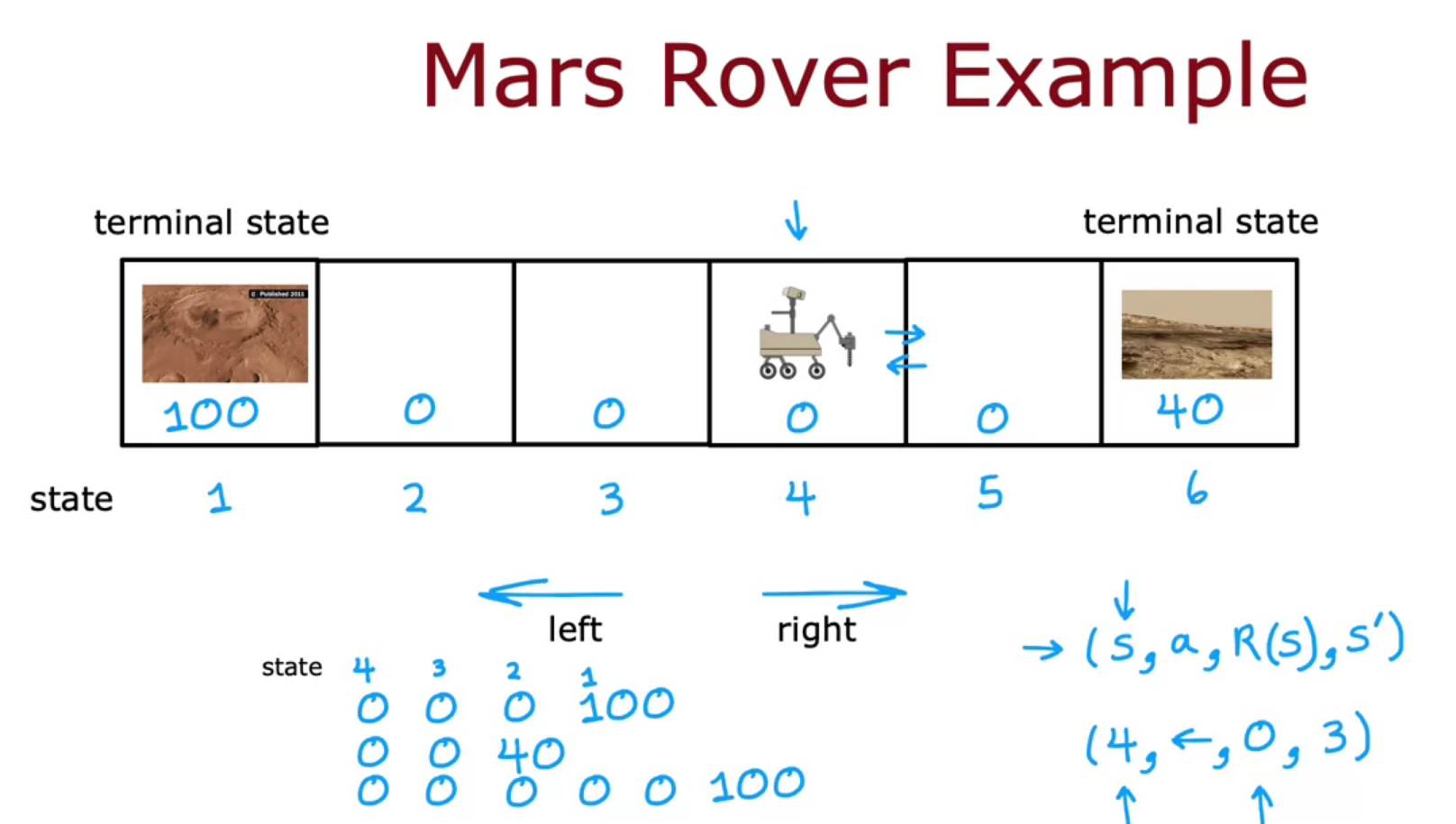
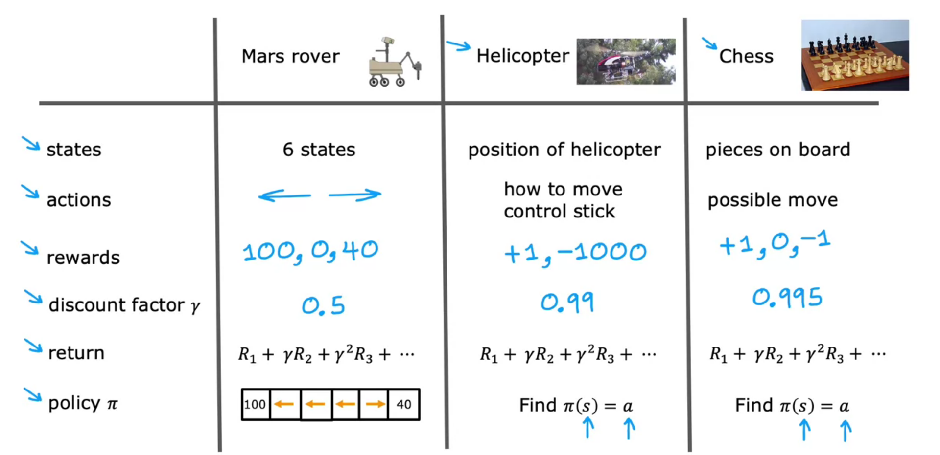
Mars Rover example
For a robot in mars trying to find water/rock/surface. The position of rover or robot is State. The reward we provide to state decide the target for the rover. It can go to left or right. The final state after which nothing happens is called Terminal State. But it will learn from mistakes.
It will have 4 values
- The current state it is having
- The action it took
- The reward it got for action
- The new state
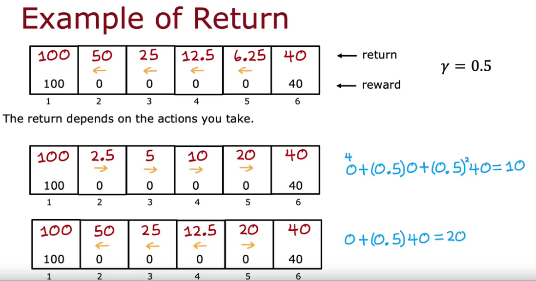
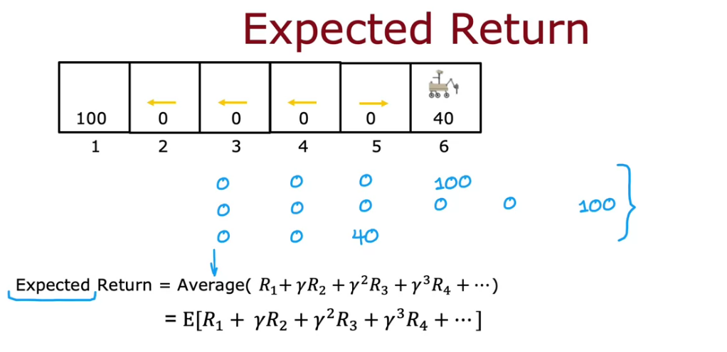
The Return in Reinforcement Learning
- We can connect Reward and Discount Factor (gamma) for reaching at final state.
- The reward value decreases as Length/Distance increases, since it takes more time to run the model.
- Discount Factor can be between 0 and 1
- Discount Factor close to 1 - Then it is really Patient to run long for reward
- Discount Factor close to 0 - Then it is really Impatient to run long for reward. It need reward fast.
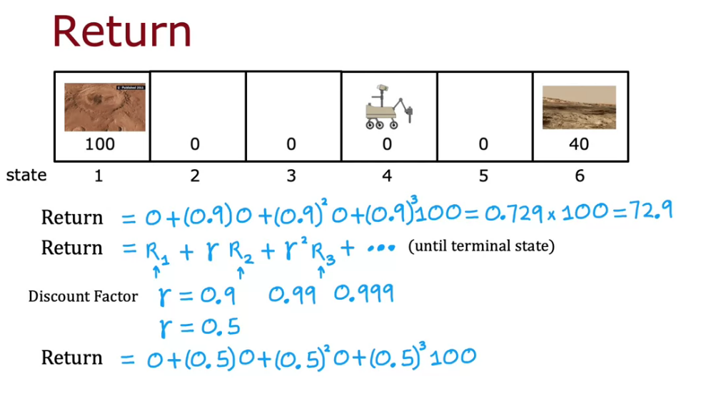
- The Return decide the Reward and Return is based on the action we take
- Return is the sum of Rewards which is weighted by the discount factor.
Making Decisions: Policies in Reinforcement Learning
- It is basically a function, which tells you to take what action to take In order to maximize the return.
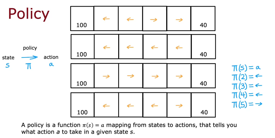
The Goal of Reinforcement Learning is to find a policy pie that tells you what actions ( a=pie(s) ) to take in every state ( s ) so as to maximize the return.
Review of Key Concepts
It is a process which defines, future depends on where you are now, not on how you got here.
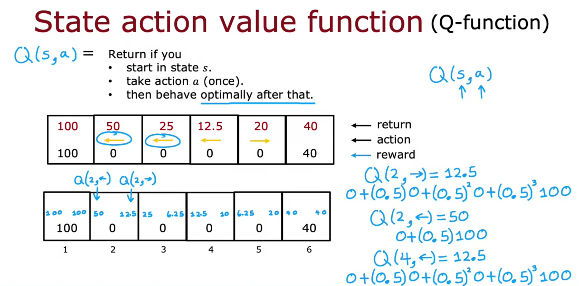
State-Action Value Function - Q Function
- It is a function denoted by Q, which depends on State and Action. Which helps us to calculate the Return
- Policy and Q is almost similar use function, with minor change
- Best Return will be Maximum of Q Function
- So best Action of State S will be action a that maximize the Q-Function

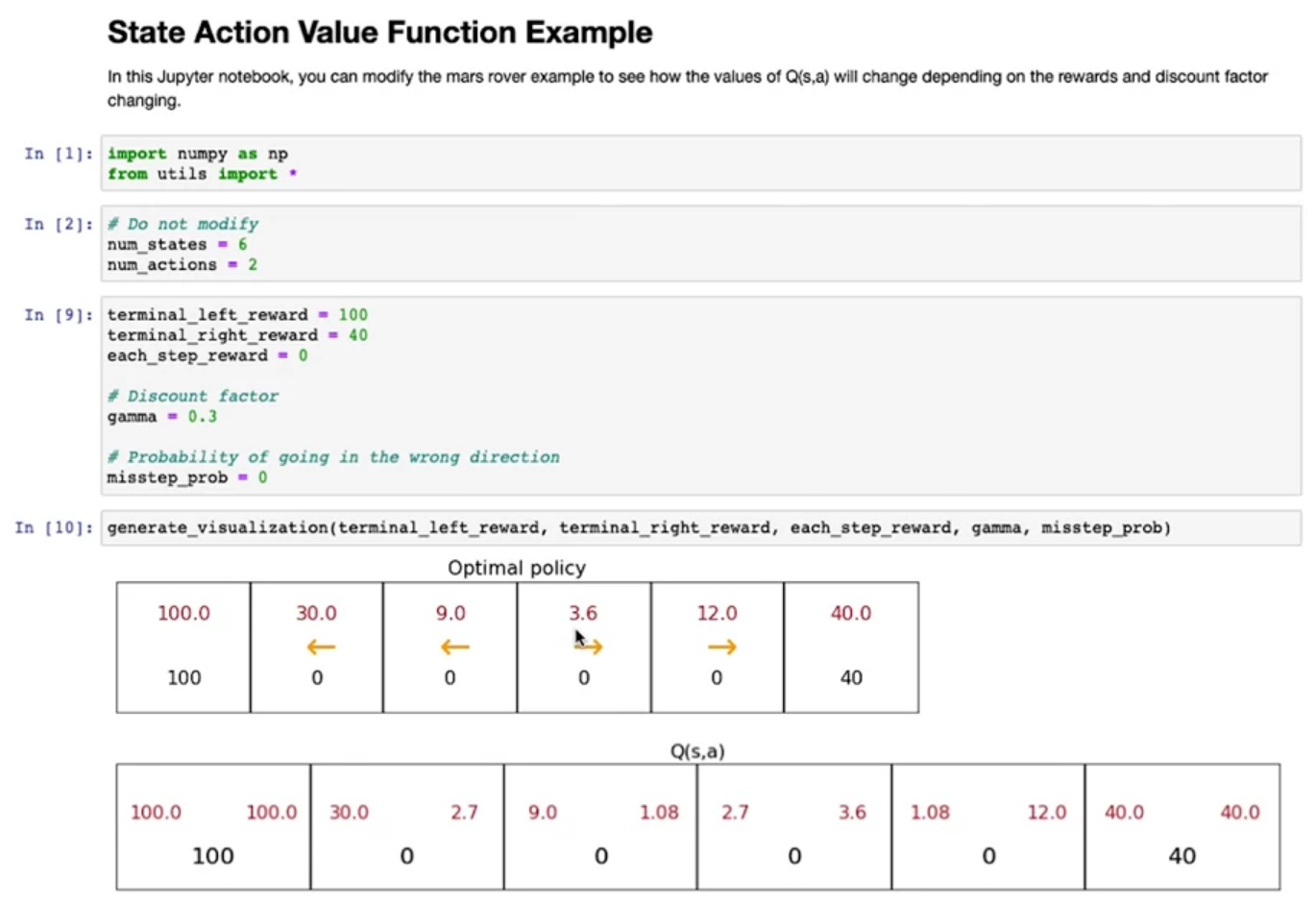
The Final Reward Value, Discount Factor (gamma) are the one depend upon the
Optimal Policy and Q -Function
Bellman Equations
- It helps us to calculate the state action value function (Q-Function)
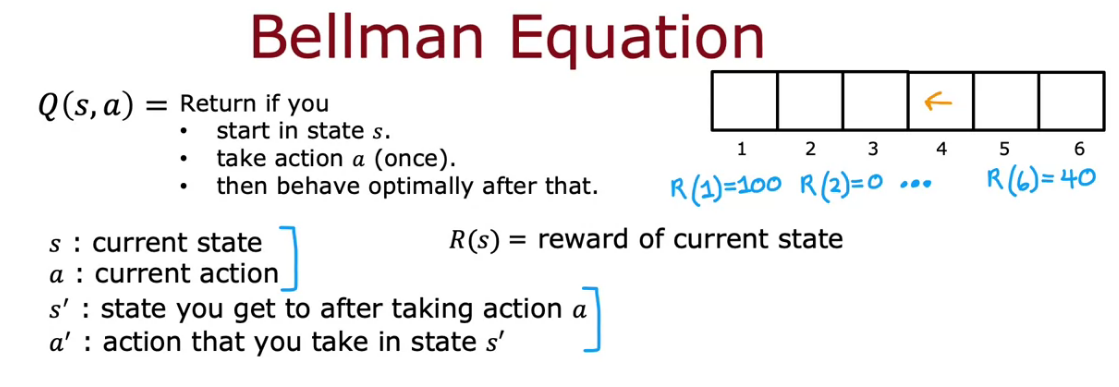


Total Return has two parts
- The reward you get right away
- The reward you get from next state due to our action
Random (Stochastic) Environment
- Suppose that the robot or problem have random output nature. A 0.1 or 10% chance to do the commands in wrong way.
- In stochastic environment there will be different rewards
- So our aim is to Maximize the Average of Sum of Discount of Rewards.
- Maximize the Expected Return
- So Bellman Equation changes with expected maximum of Q-Function

- There will be a mis-step variable in such cases
- If value of misstep is high, there will be decrease in Q-Value
- If value of misstep is low, Q-Value won’t have that much impact.
Example of continuous state space applications
- In our robot example, we have fixed state to travel. It is Discrete
- If our goal is to run a truck from 0 to 6 km, it is Continuos
- For a truck since it won’t fly. We can have 2 axis X and Y along with theta it turn, while moving in that plane.
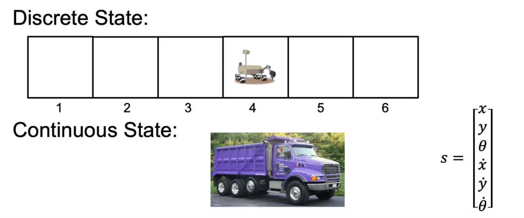
- If we are controlling a helicopter, We have X, Y, Z axis and 3 angle between XY, YZ, XZ axis

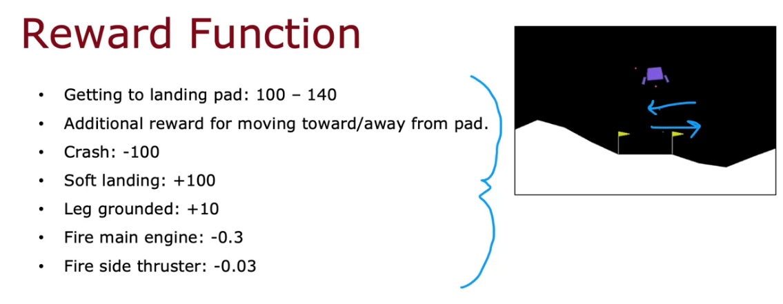
Lunar Lander
It mainly has 4 actions to do
- Do nothing
- Left Thruster
- Right Thruster
- Main Thruster
We can represent them as a vector of X, Y and tilt Theta along with the binary value l and r which represent left or right leg in ground

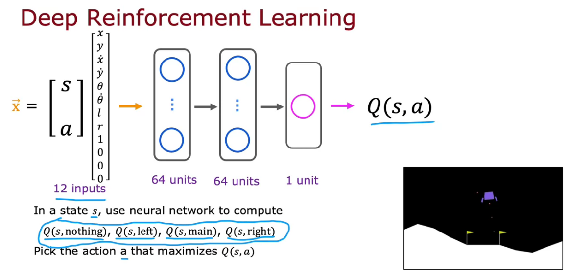
Learning the State-Value Function
- 12 inputs where 6 from the X, Y and theta before and after case, 2 for left l and right r.
- 4 for four actions represented as 1, 0, 0, 0 or 0, 1, 0, 0 like that.
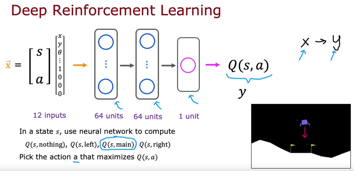
So here we apply similar to linear regression where we predict y based on a input x function
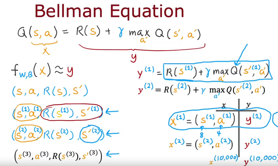
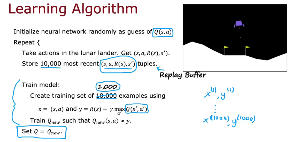
Learning Algorithm
- Initialize the NN randomly as guess of Q(s, a)
- Repeat actions and store 10000 most recent one. It is called Replay Buffer
- Train NN using the 10000 training set
- Then calculate new Q-Function
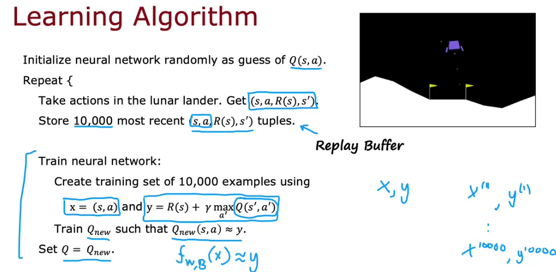
This algorithm is called DQN - Deep Q Network, we use deep learning and NN, to learn the Q-Function
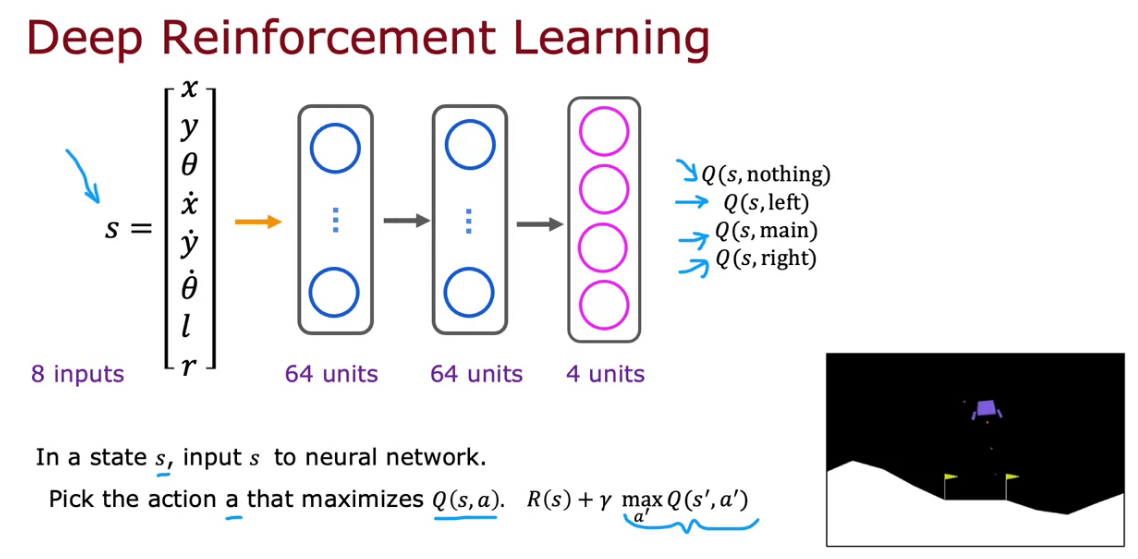
Algorithm refinement: Improved neural network architecture
The current algorithm is inefficient, because we have to carry 4 inference of action from each state.
But if we change the NN by 8 input it become much more efficient.
Algorithm refinement: ϵ-greedy policy
- In order to learn things even it’s a bad idea, random actions helps. Otherwise it will end up doing things which Maximize the Q Function and won’t be prepared for the worse.
- This idea of picking randomly is called Exploration
- 1 - Exploration is also called a Greedy Action/Exploitation Step
- It have epsilon greedy policy, which give percentage of random picking
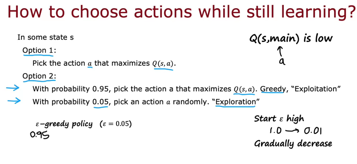
Start at high epsilon to get more random actions, slowly decrease it to learn the correct one. Learning will take more time in Reinforcement Learning, when parameters are not set in a correct way.
Algorithm Refinement: Mini-Batch and Soft Updates
- If data is huge, In Gradient Descent we need to find average and derivative in each time.
- So GD becomes slow
- We can use Mini-Batch to solve this issue
- We will pick subset of the complete data to run the GD. So it becomes fast.
It works on Supervised Learning and Reinforcement Learning
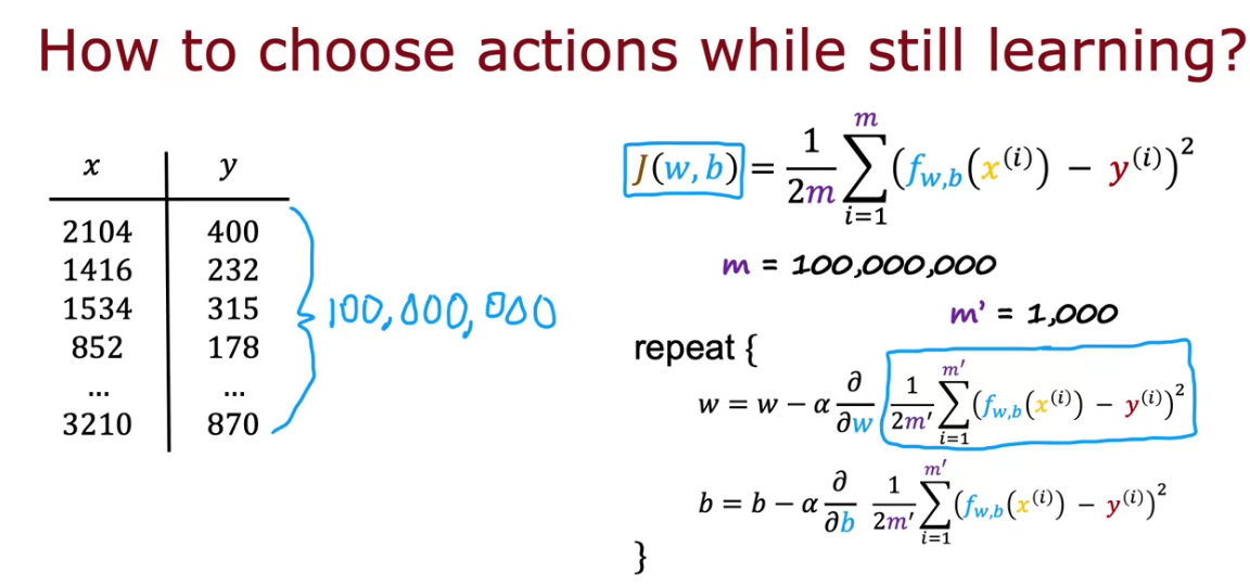


In case of training if 10000 examples are available, we only use a subset 1000 each time to become much faster, and little noisy.
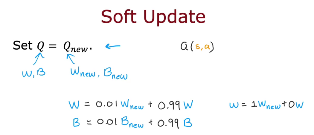
We only choose a subset with little different from the old one. We take time to learn the old things. Soft Update take care of this. We change gradually.
The State of Reinforcement Learning
Limitation
- Work easily on Game, Not in real Robot.
- Few application using RL than Supervised and Un-Supervised Learning.
- But existing research going on.
Overview
Courses
- Supervised Machine Learning: Regression and Classification
- Linear regression
- logistic regression
- gradient descent
- Advanced Learning Algorithms
- Neural networks
- decision trees
- advice for ML
- Unsupervised Learning, Recommenders, Reinforcement Learning
- Clustering
- anomaly detection
- collaborative filtering
- content based filtering
- reinforcement learning